Underwater sound propagation

Closed-form underwater propagation, complementing the reference levels of the Underwater acoustics page: the transmission loss, the speed of sound in sea water, the sonar equation, seabed reflection loss and the ocean ambient-noise spectrum.

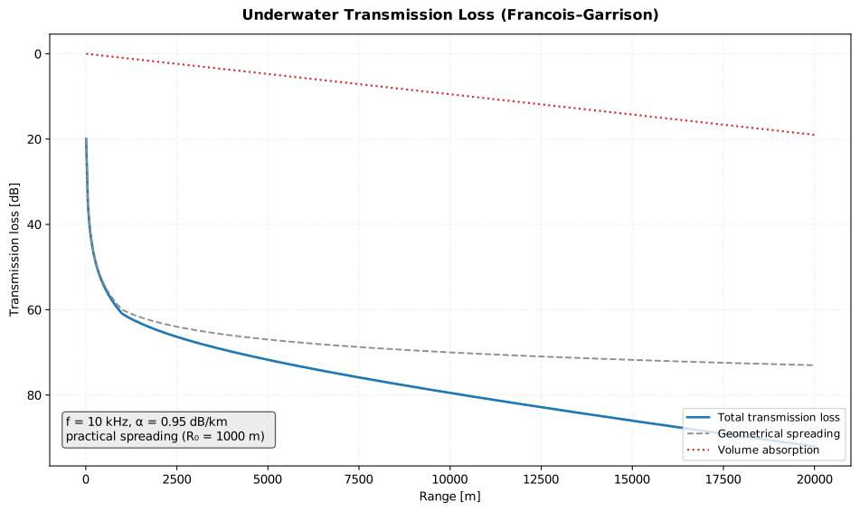
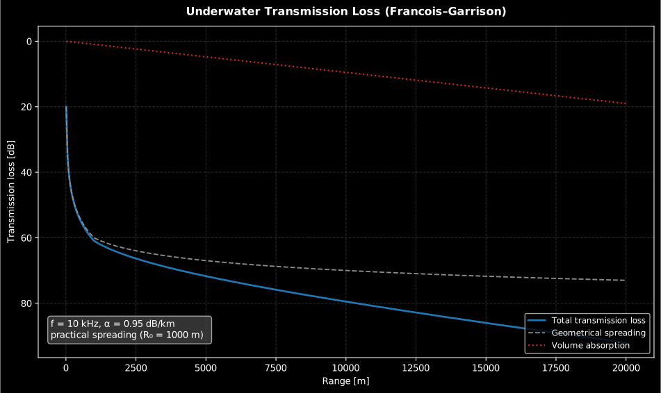
Transmission loss

The transmission loss is

$$TL=\text{spreading}+\alpha R.$$

Geometrical spreading is $20\lg R$ (spherical), $10\lg R$ (cylindrical) or spherical up to a transition range $R_0$ and cylindrical beyond it ("practical"). The volume absorption $\alpha$ (dB/km) comes from Francois–Garrison (1982, default and reference), Ainslie–McColm (1998) or Thorp (1967, frequency-only); the first two agree to within ~10 % across 100 Hz–1 MHz.

Show the code for this figure

import matplotlib.pyplot as plt
import numpy as np
from phonometry import underwater

# 10 kHz at 10 °C, 35 ppt, 100 m depth; practical spreading with R0 = 1000 m.
ranges = np.linspace(10.0, 20_000.0, 400)
tl = underwater.transmission_loss(ranges, 10e3, law="practical",
                                  transition_range=1000.0, temperature=10.0,
                                  salinity=35.0, depth=100.0)
print(f"alpha = {tl.absorption_coefficient:.2f} dB/km")   # alpha = 0.95 dB/km
tl.plot()   # total TL with the spreading and absorption contributions
plt.show()

import numpy as np
from phonometry import underwater

ranges = np.linspace(10.0, 20_000.0, 400)
tl = underwater.transmission_loss(ranges, 10e3, law="practical", transition_range=1000.0,
                          temperature=10.0, salinity=35.0, depth=100.0)
print(tl.absorption_coefficient, tl.tl[-1])
tl.plot()   # TL vs range with the spreading/absorption split (needs matplotlib)

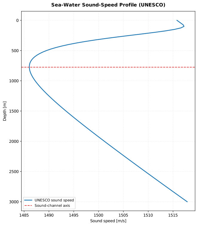
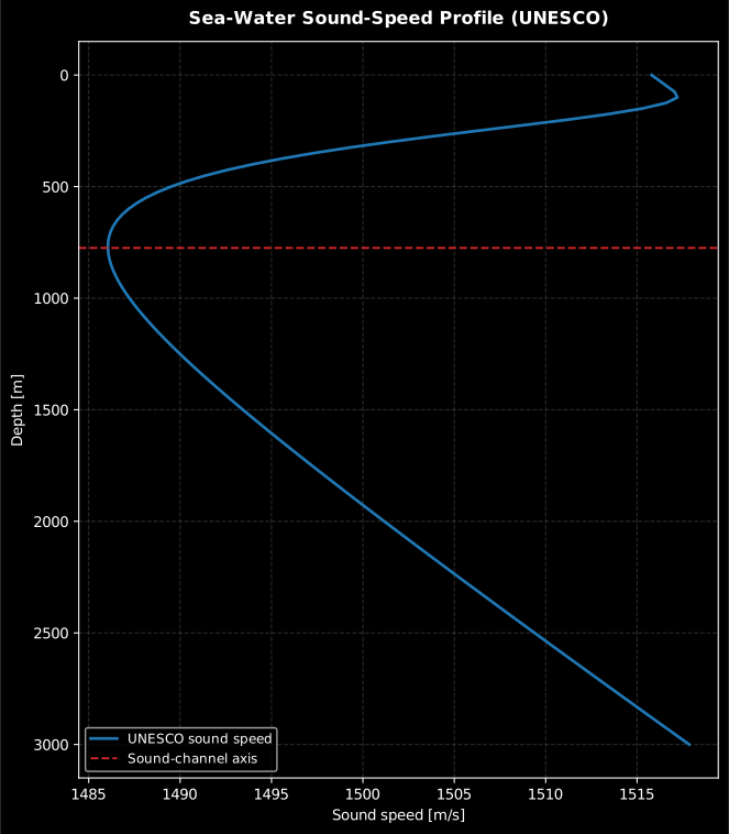
Speed of sound in sea water

sea_water_sound_speed(T, S, depth, model=…) uses the UNESCO / Chen–Millero equation (default, in the Wong & Zhu 1995 ITS-90 form), Del Grosso (1974) or Mackenzie (1981). Depth is converted to pressure with Leroy & Parthiot (1998). The three agree to within ~1 m/s; Mackenzie’s canonical check value is 1550.744 m/s at 25 °C, 35 ppt, 1000 m.

Show the code for this figure

import matplotlib.pyplot as plt
import numpy as np
from phonometry import underwater

# A warm mixed layer, a thermocline down to 4 °C and an isothermal deep layer.
depths = np.linspace(0.0, 3000.0, 121)
temps = 4.0 + 14.0 / (1.0 + (np.maximum(depths - 80.0, 0.0) / 250.0) ** 2)
profile = underwater.sound_speed_profile(depths, temps, 35.0, model="unesco")
profile.plot()   # sound speed vs depth, minimum at the sound-channel axis
plt.show()

import numpy as np
from phonometry import underwater

c = underwater.sea_water_sound_speed(25.0, 35.0, 1000.0, model="mackenzie")  # 1550.744
depths = np.linspace(0.0, 3000.0, 121)
temps = 4.0 + 14.0 / (1.0 + (np.maximum(depths - 80.0, 0.0) / 250.0) ** 2)
profile = underwater.sound_speed_profile(depths, temps, 35.0, model="unesco")
profile.plot()   # sound speed vs depth (needs matplotlib)

The $c(z)$ minimum acts as a waveguide (the SOFAR channel): wavefronts that stray from the axis are refracted back toward it, while sound generated outside the channel leaks away to depth, as the simulation below shows with an intentionally exaggerated gradient. This trapping is why low-frequency sound can cross entire oceans.

Two 2D FDTD runs of a low-frequency pulse in a SOFAR-like underwater sound channel, with the c(z) profile drawn beside each field. Launched on the channel axis at 400 m depth the wavefronts keep refracting back toward the sound-speed minimum and stay trapped; launched near the surface at 150 m the energy crosses the channel and leaks away to depth. The closing seconds fade to the time-integrated energy map, showing the whole path history of each run.

Download the animation (WebM)

Two 2D FDTD runs of a low-frequency pulse in a SOFAR-like underwater sound channel, with the c(z) profile drawn beside each field. Launched on the channel axis at 400 m depth the wavefronts keep refracting back toward the sound-speed minimum and stay trapped; launched near the surface at 150 m the energy crosses the channel and leaks away to depth. The closing seconds fade to the time-integrated energy map, showing the whole path history of each run.

Download the animation (WebM)

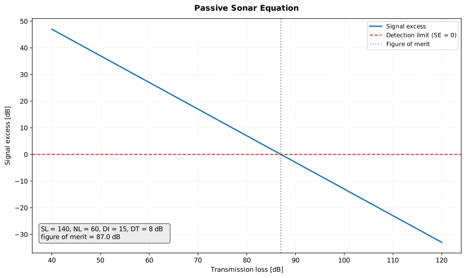
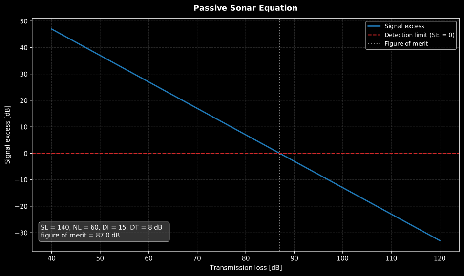
Sonar equation

The sonar equation gives the signal excess $SE$ (detection when $SE\ge 0$) and the figure of merit (the maximum allowable transmission loss at $SE=0$):

$$SE=SL-TL-(NL-DI)-DT\text{(passive)},$$ $$SE=SL-2TL+TS-(NL-DI)-DT\text{(active, monostatic)},$$

or reverberation-limited with $RL$ in place of $NL-DI$.

Show the code for this figure

import matplotlib.pyplot as plt
import numpy as np
from phonometry import underwater

tl = np.linspace(40.0, 120.0, 400)
se = underwater.passive_sonar_equation(source_level=140.0, transmission_loss=tl,
                                       noise_level=60.0, directivity_index=15.0,
                                       detection_threshold=8.0)
print(f"figure of merit = {se.figure_of_merit:.1f} dB")  # figure of merit = 87.0 dB
se.plot()   # signal excess vs transmission loss, zero crossing at the FOM
plt.show()

import numpy as np
from phonometry import underwater

tl = np.linspace(40.0, 120.0, 400)
se = underwater.passive_sonar_equation(source_level=140.0, transmission_loss=tl,
                               noise_level=60.0, directivity_index=15.0,
                               detection_threshold=8.0)
print(se.figure_of_merit)
se.plot()   # signal excess vs transmission loss (needs matplotlib)

Sonar, propagation and ambient levels are in dB re a plane wave of 1 µPa rms (spectrum levels). Source levels (below) use the source convention, dB re 1 µPa²/Hz at 1 m.

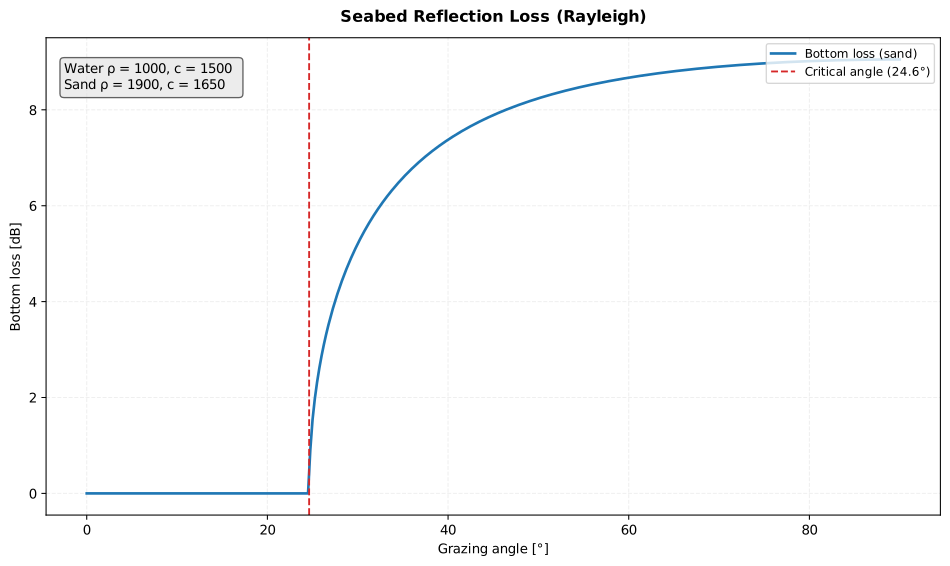
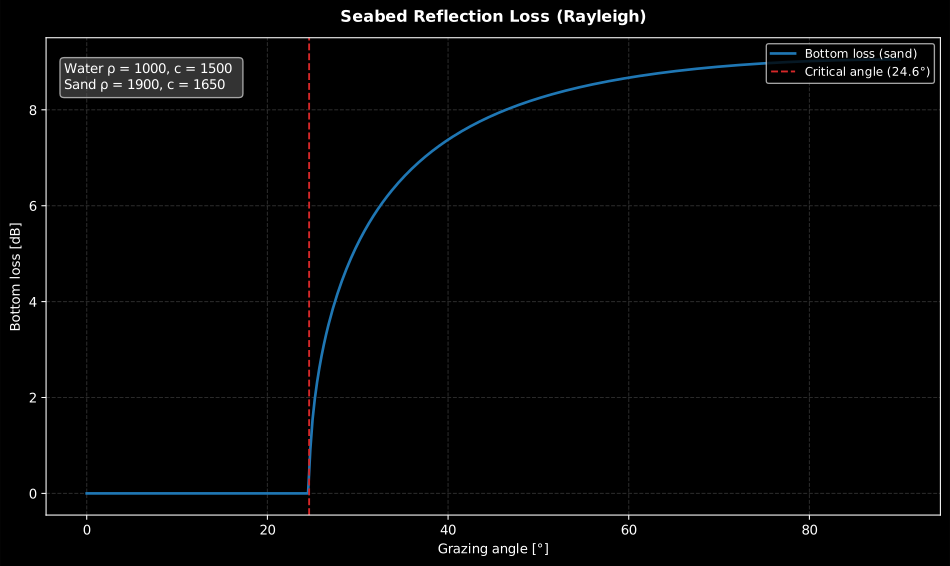
Seabed reflection loss

A plane wave striking the seabed reflects with the fluid–fluid Rayleigh reflection coefficient (Medwin & Clay). For a faster bottom ($c_2>c_1$) there is a critical grazing angle ${\phi }_c=\arccos (c_1/c_2)$, below which the wave is totally reflected ($|R|=1$, zero loss). The bottom loss is $BL=-20\lg |R|$.

Show the code for this figure

import matplotlib.pyplot as plt
import numpy as np
from phonometry import underwater

# Rayleigh fluid-fluid reflection: water over a fast sandy bottom.
phi = np.linspace(0.0, 90.0, 361)
bl = underwater.bottom_reflection_loss(phi, rho1=1000.0, c1=1500.0,
                                       rho2=1900.0, c2=1650.0)
print(f"critical angle = {bl.critical_angle:.1f} deg")   # critical angle = 24.6 deg
bl.plot()   # bottom loss vs grazing angle
plt.show()

import numpy as np
from phonometry import underwater

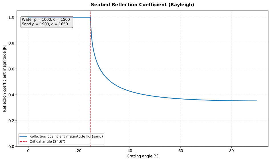
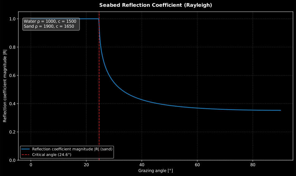
phi = np.linspace(0.0, 90.0, 361)   # grazing angle from the interface, degrees
bl = underwater.bottom_reflection_loss(phi, rho1=1000.0, c1=1500.0,   # water
                               rho2=1900.0, c2=1650.0)          # sand
print(bl.critical_angle)            # 24.6°
bl.plot()   # bottom loss vs grazing angle (needs matplotlib)

The companion seabed_reflection bundles the complex reflection_coefficient, its magnitude $|R|$, the bottom_loss (dB) and the interface parameters into a SeabedReflection whose .plot() draws the reflection-coefficient magnitude $|R|$ directly (unity below the critical angle, dropping to the normal-incidence value at $90°$).

Show the code for this figure

import matplotlib.pyplot as plt
import numpy as np
from phonometry import underwater

# Rayleigh reflection-coefficient magnitude: water over a fast sandy bottom.
phi = np.linspace(0.0, 90.0, 361)
sr = underwater.seabed_reflection(phi, rho1=1000.0, c1=1500.0,
                                  rho2=1900.0, c2=1650.0)
print(f"|R| at normal incidence = {sr.magnitude[-1]:.3f}")  # 0.353
sr.plot()   # reflection-coefficient magnitude vs grazing angle
plt.show()

import numpy as np
from phonometry import underwater

phi = np.linspace(0.0, 90.0, 361)   # grazing angle from the interface, degrees
sr = underwater.seabed_reflection(phi, rho1=1000.0, c1=1500.0,   # water
                          rho2=1900.0, c2=1650.0)          # sand
print(sr.magnitude[-1])             # 0.353 = |R| at normal incidence
sr.plot()   # |R| vs grazing angle (needs matplotlib)

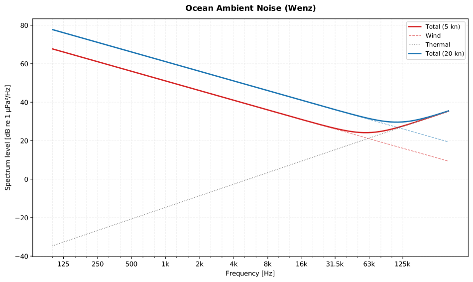
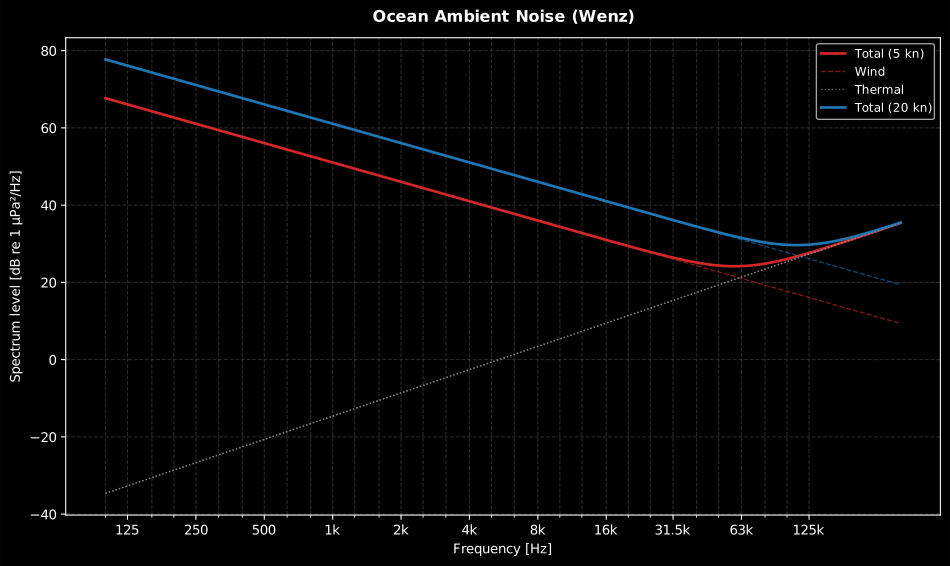
Ocean ambient noise

The ambient-noise spectrum level is the energy sum of the physically grounded Wenz components: wind / sea-surface noise via the “rule of fives” (the historical 25 dB anchor at 1 kHz for 5 knots is re 20 µPa, i.e. ~51 dB re 1 µPa; strictly valid ~500 Hz–5 kHz) and Mellen thermal noise (dominant above ~50 kHz). The wide example range keeps the wind curve plotted beyond ~5 kHz only as an extrapolation to show the thermal crossover. A shipping spectrum may be supplied by the caller.

Show the code for this figure

import matplotlib.pyplot as plt
import numpy as np
from phonometry import underwater

# Wenz ambient noise (wind rule of fives + Mellen thermal) at two wind speeds.
freqs = np.logspace(2, 5.5, 300)
fig, ax = plt.subplots()
for u in (5.0, 20.0):
    noise = underwater.ocean_ambient_noise(freqs, wind_speed_knots=u)
    ax.semilogx(noise.frequency, noise.spectrum_level, label=f"Total ({u:.0f} kn)")
ax.semilogx(freqs, underwater.thermal_noise_spectrum(freqs), ":", label="Thermal")
ax.set(xlabel="Frequency [Hz]", ylabel="Spectrum level [dB re 1 µPa²/Hz]")
ax.legend()
ax.grid(True, which="both", alpha=0.3)
plt.show()

import numpy as np
from phonometry import underwater

freqs = np.logspace(2, 5.5, 300)
noise = underwater.ocean_ambient_noise(freqs, wind_speed_knots=15.0)
noise.plot()   # composite spectrum with wind/thermal components (needs matplotlib)

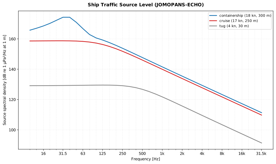
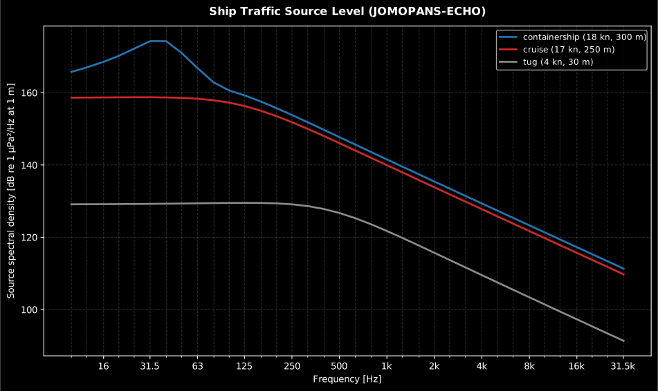
Ship-traffic source level

When no measured spectrum is available, a ship’s source level can be estimated from its class, speed and length with JOMOPANS-ECHO (MacGillivray & de Jong 2021, the default, validated against 1862 measurements), RANDI 3.1 or Wales & Heitmeyer (2002).

Show the code for this figure

import matplotlib.pyplot as plt
from phonometry import underwater

# JOMOPANS-ECHO source spectra for three vessel classes (speed, length).
fig, ax = plt.subplots()
for vessel_class, speed, length in (("containership", 18.0, 300.0),
                                    ("cruise", 17.1, 250.0),
                                    ("tug", 3.7, 30.0)):
    s = underwater.ship_source_spectrum(speed, length, vessel_class=vessel_class)
    ax.semilogx(s.frequency, s.source_psd,
                label=f"{vessel_class} ({speed:.0f} kn, {length:.0f} m)")
ax.set(xlabel="Frequency [Hz]",
       ylabel="Source spectral density [dB re 1 µPa²/Hz at 1 m]")
ax.legend()
ax.grid(True, which="both", alpha=0.3)
plt.show()

from phonometry import underwater

ship = underwater.ship_source_spectrum(18.0, 300.0, vessel_class="containership")
ship.plot()                     # source spectral density vs frequency
print(underwater.VESSEL_CLASSES)        # the 13 JOMOPANS-ECHO vessel classes

# Feed the prediction into the ambient noise as the shipping term:
noise = underwater.ocean_ambient_noise(ship.frequency, wind_speed_knots=10.0,
                               shipping=ship.source_psd)

Numerical solvers

For range-independent environments the field can be computed numerically with three solvers (Jensen et al., Computational Ocean Acoustics):

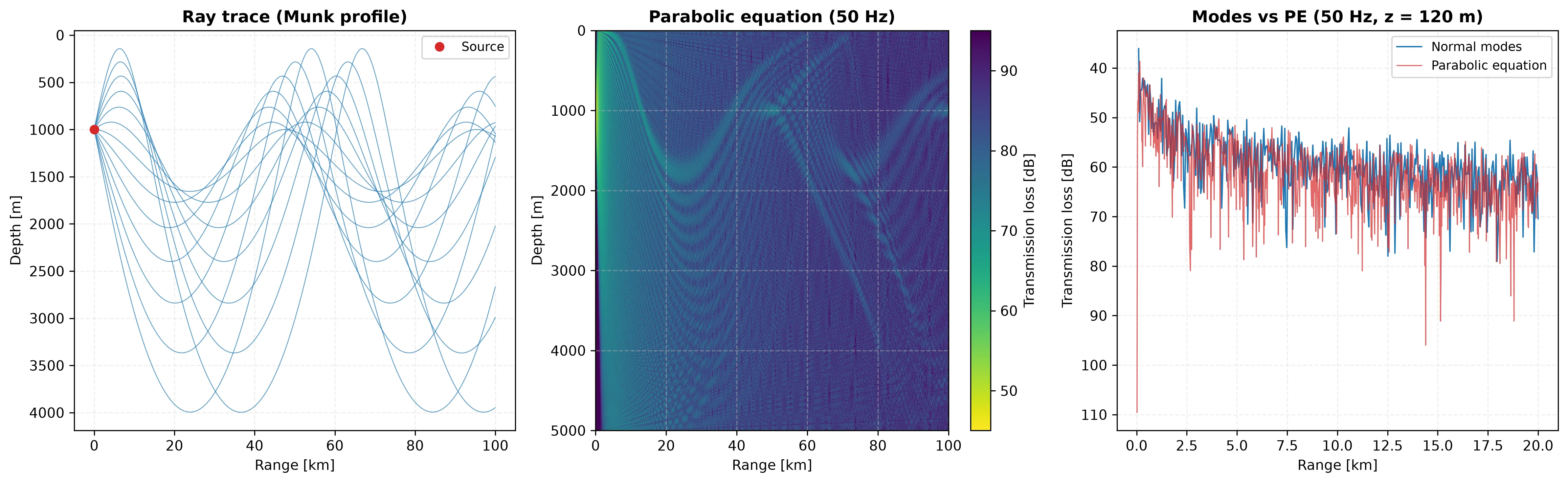
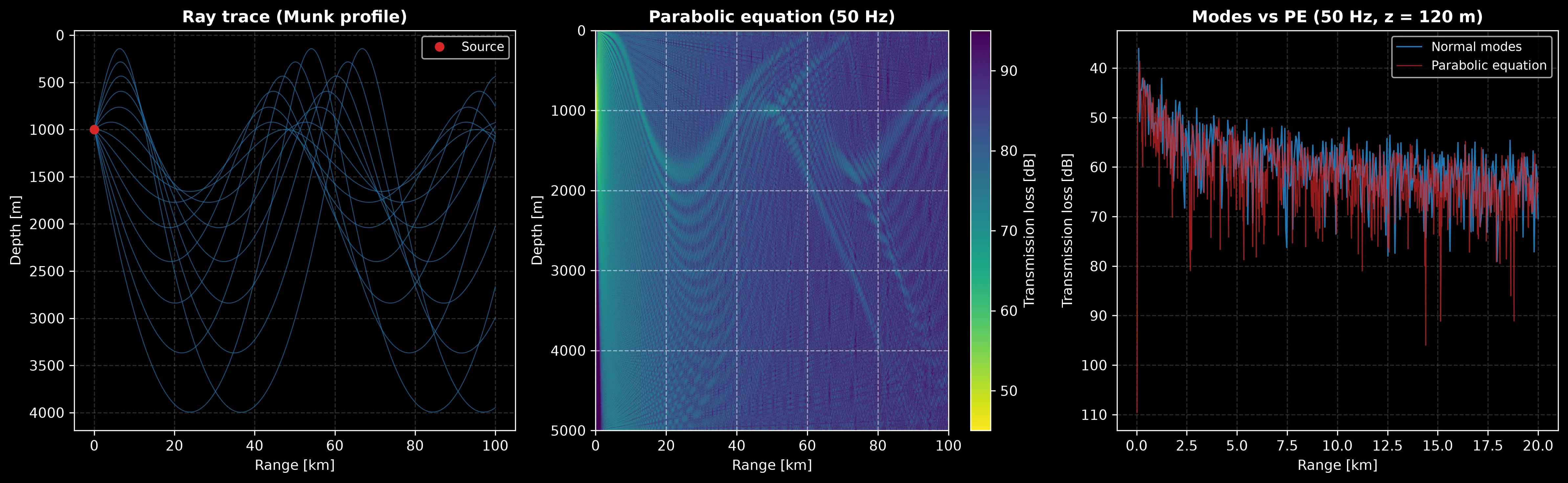
• normal_modes: the depth-separated Sturm-Liouville eigenproblem solved by finite differences, summed into transmission loss (validated against the ideal waveguide’s exact modes).
• ray_trace: the ray-trajectory equations integrated with Runge-Kutta, vectorised over all rays at once (validated against a linear gradient’s circular arcs).
• parabolic_equation: the standard (Tappert) PE via the split-step Fourier algorithm (validated against free-field spherical spreading).

Show the code for this figure

import matplotlib.pyplot as plt
import numpy as np
from phonometry import underwater

# A Munk deep-water sound-speed profile.
z = np.linspace(0.0, 5000.0, 60)
eta = 2.0 * (z - 1300.0) / 1300.0
c = 1500.0 * (1.0 + 0.00737 * (eta - 1.0 + np.exp(-eta)))

# Split-step Fourier PE at 50 Hz; a coarse grid keeps the run fast.
field = underwater.parabolic_equation(50.0, z, c, source_depth=1000.0,
                                      max_range=50_000.0, range_step=50.0,
                                      n_depth_points=512)
field.plot()   # TL(z, r) field showing the convergence zones
plt.show()

import numpy as np
from phonometry import underwater

z = np.linspace(0.0, 5000.0, 60)
eta = 2.0 * (z - 1300.0) / 1300.0
c = 1500.0 * (1.0 + 0.00737 * (eta - 1.0 + np.exp(-eta)))   # Munk profile
underwater.ray_trace(z, c, source_depth=1000.0,
             launch_angles_deg=np.linspace(-12, 12, 21), max_range=100e3).plot()

modes = underwater.normal_modes(50.0, [0.0, 200.0], [1500.0, 1500.0],
                        source_depth=50.0, receiver_depth=100.0)
underwater.parabolic_equation(50.0, [0.0, 200.0], [1500.0, 1500.0],
                      source_depth=50.0, max_range=20e3).plot()

All three assume a range-independent water column with a pressure-release surface.

Choosing a model

Every function above answers the same question, “how much level survives the path”, at a different price in physics. Terminology throughout follows ISO 18405:2017 (propagation loss, source level, levels re 1 µPa).

Sound speed. The three equations agree to within about 1 m/s inside their common domain, so the choice is about validity range, not accuracy. The default UNESCO / Chen-Millero form (as recast by Wong & Zhu 1995) covers 0–40 °C, 0–40 ppt and 0–1000 bar, the widest envelope, and is the international standard. Del Grosso (1974) is restricted to 0–30 °C and 30–40 ppt but is preferred by some authors for deep-ocean work inside that domain (much of the SOFAR-channel literature uses it). Mackenzie (1981) trades pressure for depth directly (2–30 °C, 25–40 ppt, 0–8000 m), which makes it the convenient choice when you have an echo-sounder depth rather than a CTD pressure; the other two convert depth to pressure through Leroy & Parthiot (1998) internally.

Absorption. Francois–Garrison (1982) is the reference and the default: it carries the boric-acid, magnesium-sulfate and pure-water relaxations with their full temperature, salinity, depth and pH-implicit dependences, and is trusted from about 100 Hz to 1 MHz. Ainslie–McColm (1998) is a deliberate simplification of the same physics that stays within about 10 % of it across that range; use it when a legible formula matters more than the last percent. Thorp (1967) depends on frequency only (it bakes in 4 °C water near 1000 m) and predates both; keep it for quick low-frequency estimates below a few tens of kHz and for comparison with older literature that used it.

Spreading law. Spherical spreading ($20\lg R$) describes a wavefront that expands freely in three dimensions, before any boundary confines it; cylindrical spreading ($10\lg R$) describes energy trapped between the surface and the bottom (or in the SOFAR channel) that can only expand in range. The "practical" law splices the two at a transition range $R_0$, which is physically of the order of the water (or channel) depth: spherical while the wavefront has not yet filled the duct, cylindrical once it has. In the 10 kHz example above the choice is not cosmetic: against the same figure of merit of 87 dB, spherical-only spreading predicts detection out to about 8.7 km while the practical law with $R_0=1000$ m stretches it to about 15.8 km. When the spreading law is the biggest uncertainty in the budget, that is the cue to stop using a closed form and compute the field.

Closed form or solver. The closed-form transmission loss knows nothing of the sound-speed profile, the seabed or the surface; it is honest for short, direct, boundary-free paths and for first-cut sonar budgets. When refraction and boundaries decide the answer, pick the solver by frequency and geometry (Jensen et al. 2011, Ch. 1):

Solver	Natural regime	What it buys you
ray_trace	High frequency (water depth ≫ λ), deep water	Eigenray geometry, travel times, convergence zones; cost independent of frequency
normal_modes	Low frequency, shallow water, range-independent	Finite-difference modal sum with few propagating modes ($m<kD/\pi$); the reference solution for its regime, validated against the ideal waveguide’s exact modes
parabolic_equation	Low frequency, long one-way paths	Full-field TL($z$,$r$) with refraction, marched in range over the range-independent $c(z)$ all three solvers assume

The boundaries blur in practice: rays remain usable at surprisingly low frequencies for travel-time work, and the PE remains the workhorse well above its formal small-angle regime. When two of the three agree on a case, as the modes and the PE do in the figure above, that agreement is the practical convergence test.

A worked sonar budget. Chain the pieces end to end: a 140 dB re 1 µPa²/Hz source at 10 kHz, a 60 dB ambient spectrum level, a 15 dB array gain and an 8 dB detection threshold give the figure of merit $FOM=140-(60-15)-8=87$ dB computed by passive_sonar_equation above. The transmission-loss curve of the first section (10 °C, 35 ppt, 100 m, $\alpha =0.95$ dB/km) crosses 87 dB at about 15.8 km with the practical law: that crossing is the predicted detection range, and every term of the budget moves it. Trim the directivity index to 7.5 dB and the figure of merit falls to 79.5 dB, so the range drops to wherever the TL curve crosses that value; double the frequency to 20 kHz and $\alpha$ more than triples to 3.3 dB/km, pulling the crossing sharply inward. This coupling between the absorption model, the spreading law and the sonar equation is why the three live in one module.

What this guide covers

Covered. ISO 18405:2017 terminology (propagation loss, source level, levels re 1 µPa) underlies every quantity on this page. transmission_loss and seawater_absorption implement geometrical spreading plus the Francois-Garrison (1982, default), Ainslie-McColm (1998) or Thorp (1967) absorption models. sea_water_sound_speed and sound_speed_profile implement the UNESCO/Chen-Millero (Wong & Zhu 1995 ITS-90 form, default), Del Grosso (1974) and Mackenzie (1981) sound-speed equations, with the Leroy & Parthiot (1998) depth-to-pressure conversion. passive_sonar_equation and active_sonar_equation implement the passive and monostatic active sonar equations (Urick, via Etter 2003). seabed_reflection and bottom_reflection_loss implement the fluid-fluid Rayleigh reflection coefficient and critical angle (Medwin & Clay). ocean_ambient_noise sums the Wenz wind “rule of fives” and Mellen thermal-noise components. ship_source_spectrum implements the JOMOPANS-ECHO (default), RANDI 3.1 and Wales & Heitmeyer (2002) source-level models. normal_modes, ray_trace and parabolic_equation implement the Jensen et al. (2011) numerical solvers.

Not covered. The seabed model is lossless fluid-fluid Rayleigh reflection only, so sediment attenuation is out of scope. normal_modes, ray_trace and parabolic_equation assume a range-independent water column with a pressure-release or rigid boundary only, not an absorbing or elastic bottom, so real bathymetry is not modelled. active_sonar_equation is monostatic only: there is no bistatic geometry. ocean_ambient_noise leaves out the low-frequency turbulence band and any built-in distant-shipping model; supply a shipping spectrum yourself, for instance from ship_source_spectrum above.

See also

• API reference: underwater.propagation, underwater.numerical_propagation and underwater.sound_speed.

References

• Ainslie, M. A., & McColm, J. G. (1998). A simplified formula for viscous and chemical absorption in sea water. The Journal of the Acoustical Society of America, 103(3), 1671-1672. https://doi.org/10.1121/1.421258The legible simplified absorption model ("ainslie-mccolm").
• Carey, W. M., & Evans, R. B. (2011). Ocean ambient noise: Measurement and theory. Springer. https://doi.org/10.1007/978-1-4419-7832-5The wind "rule of fives" anchor and the Mellen thermal-noise derivation.
• Chen, C.-T., & Millero, F. J. (1977). Speed of sound in seawater at high pressures. The Journal of the Acoustical Society of America, 62(5), 1129-1135. https://doi.org/10.1121/1.381646The UNESCO international-standard sound-speed equation.
• Del Grosso, V. A. (1974). New equation for the speed of sound in natural waters (with comparisons to other equations). The Journal of the Acoustical Society of America, 56(4), 1084-1091. https://doi.org/10.1121/1.1903388The alternative pressure-based sound-speed equation ("del-grosso").
• Francois, R. E., & Garrison, G. R. (1982). Sound absorption based on ocean measurements: Part I: Pure water and magnesium sulfate contributions. The Journal of the Acoustical Society of America, 72(3), 896-907. https://doi.org/10.1121/1.388170The pure-water and magnesium-sulfate halves of the default absorption model of the transmission-loss section.
• Francois, R. E., & Garrison, G. R. (1982). Sound absorption based on ocean measurements. Part II: Boric acid contribution and equation for total absorption. The Journal of the Acoustical Society of America, 72(6), 1879-1890. https://doi.org/10.1121/1.388673The boric-acid term and the complete Francois-Garrison total-absorption equation, the implemented default.
• International Organization for Standardization. (2017). Underwater acoustics — Terminology (ISO 18405:2017). The standardized definitions (propagation loss, source level, sound pressure level re 1 µPa) behind the quantities of this page.
• Jensen, F. B., Kuperman, W. A., Porter, M. B., & Schmidt, H. (2011). Computational ocean acoustics (2nd ed.). Springer. https://doi.org/10.1007/978-1-4419-8678-8The normal-mode (Ch. 5), ray-tracing (Ch. 3) and split-step Fourier parabolic-equation (Ch. 6) solvers of the numerical-solvers section, and the model-selection guidance of Ch. 1.
• Leroy, C. C., & Parthiot, F. (1998). Depth-pressure relationships in the oceans and seas. The Journal of the Acoustical Society of America, 103(3), 1346-1352. https://doi.org/10.1121/1.421275The depth-to-pressure conversion feeding the UNESCO and Del Grosso equations.
• MacGillivray, A., & de Jong, C. (2021). A reference spectrum model for estimating source levels of marine shipping based on automated identification system data. Journal of Marine Science and Engineering, 9(4), 369. https://doi.org/10.3390/jmse9040369The JOMOPANS-ECHO ship source-level model (open access); its File S1 calculator is the validation oracle.
• Mackenzie, K. V. (1981). Nine-term equation for sound speed in the oceans. The Journal of the Acoustical Society of America, 70(3), 807-812. https://doi.org/10.1121/1.386920The depth-based nine-term equation and its 1550.744 m/s check value.
• Medwin, H., & Clay, C. S. (1998). Fundamentals of acoustical oceanography. Academic Press. ISBN 978-0-12-487570-8. The fluid-fluid Rayleigh reflection coefficient and critical grazing angle of the seabed-reflection section.
• Thorp, W. H. (1967). Analytic description of the low-frequency attenuation coefficient. The Journal of the Acoustical Society of America, 42(1), 270. https://doi.org/10.1121/1.1910566The frequency-only low-frequency absorption formula ("thorp").
• Urick, R. J. (1983). Principles of underwater sound (3rd ed.). McGraw-Hill. Reprinted 1996 by Peninsula Publishing. ISBN 978-0-932146-62-5. Open Library record (https://openlibrary.org/books/OL9317725M). The sonar-equation framework (signal excess, figure of merit).
• Wales, S. C., & Heitmeyer, R. M. (2002). An ensemble source spectra model for merchant ship-radiated noise. The Journal of the Acoustical Society of America, 111(3), 1211-1231. https://doi.org/10.1121/1.1427355The ensemble merchant-ship spectrum model of the ship-traffic section.
• Wenz, G. M. (1962). Acoustic ambient noise in the ocean: Spectra and sources. The Journal of the Acoustical Society of America, 34(12), 1936-1956. https://doi.org/10.1121/1.1909155The ambient-noise survey behind the wind and thermal components of the ocean ambient-noise section.
• Wong, G. S. K., & Zhu, S. (1995). Speed of sound in seawater as a function of salinity, temperature, and pressure. The Journal of the Acoustical Society of America, 97(3), 1732-1736. https://doi.org/10.1121/1.413048The ITS-90 recast of the UNESCO coefficients, the implemented form.