Electroacoustics: distortion and frequency response

Two staples of audio-equipment characterisation, from a captured signal: how much an amplifier or transducer distorts a test tone, and what frequency response an input/output measurement reveals. This page covers the IEC 60268-3 distortion set: total and nth-order harmonic distortion, THD+N and SINAD through the AES17 measurement bandwidth, the per-order modulation and difference-frequency intermodulation, dynamic intermodulation (DIM) and the ITU-R 468 weighted THD, and the Bendat & Piersol frequency-response estimators H1/H2 with the ordinary coherence γ². Every quantity has an exact analytic oracle (synthetic signals with known harmonic and intermodulation amplitudes, a clipped-sine Fourier oracle, a full DIM test-signal synthesis, and a known LTI path), so the numbers are verifiable rather than tuned. The closing sections cover the sensitivity conventions of IEC 60268-4 (microphones) and IEC 60268-5 (loudspeakers), where most cross-datasheet comparisons go wrong, the baffled-piston radiation model behind loudspeaker directivity, and the IEC 60268-5 loudspeaker and IEC 60268-4 microphone rated-characteristics reports that render the standards’ data sheets from a measured response.

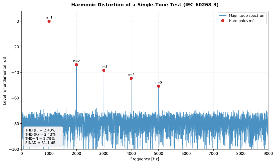
1. Harmonic distortion (IEC 60268-3 14.12.2–5)

A non-linear device fed a pure sine at f₁ returns the fundamental plus harmonics at 2f₁, 3f₁, …. The total harmonic distortion combines the harmonic amplitudes aₙ, either relative to the fundamental (kind='F') or to the total RMS (kind='R'):

$${\mathrm{THD}}_F=\frac{\sqrt{{\sum }_{n\ge 2}{a}_n^2}}{a_1},{\mathrm{THD}}_R=\frac{\sqrt{{\sum }_{n\ge 2}{a}_n^2}}{\sqrt{{\sum }_{n\ge 1}{a}_n^2}},d_n=\frac{a_n}{\sqrt{{\sum }_{k\ge 1}{a}_k^2}}.$$

dₙ is the nth-order harmonic distortion (the nth harmonic relative to the total). The tones should fall on FFT bins: use coherent sampling (an integer number of periods) or a low-leakage window so the amplitudes are read without spectral leakage.

from phonometry import electroacoustics

thd_f = electroacoustics.thd(signal, fs, 1000.0, kind="F")          # relative to fundamental
thd_r = electroacoustics.thd(signal, fs, 1000.0, kind="R")          # relative to total RMS
d2 = electroacoustics.harmonic_distortion(signal, fs, 1000.0, 2)    # 2nd-order harmonic

harmonic_analysis bundles the fundamental, the harmonic amplitudes and the THD (both conventions), THD+N and SINAD into one plottable result:

from phonometry import electroacoustics

res = electroacoustics.harmonic_analysis(signal, fs, 1000.0)
print(res.thd_f, res.thd_r, res.thd_plus_noise, res.sinad_db)
res.plot()   # annotated harmonic spectrum (needs matplotlib)

Show the code for this figure

import matplotlib.pyplot as plt
import numpy as np
from phonometry import electroacoustics

fs = 48000
n = fs                     # 1 s -> 1 Hz bins; harmonics land on bins
t = np.arange(n) / fs
f0 = 1000.0
amps = {1: 1.0, 2: 0.02, 3: 0.012, 4: 0.006, 5: 0.003}
sig = sum(a * np.sin(2 * np.pi * k * f0 * t) for k, a in amps.items())
sig = sig + np.random.default_rng(2026).standard_normal(n) * 1.2e-2

res = electroacoustics.harmonic_analysis(sig, fs, f0, n_harmonics=len(amps))
res.plot()
plt.show()

2. THD+N and SINAD (AES17-2015 6.3)

Where THD counts only the harmonics, THD+N compares everything but the fundamental (harmonics and noise) with the total signal. AES17 removes the fundamental with a standard notch filter (1.2 ≤ Q ≤ 3, validated on the applied zero-phase response per clause 5.2.8) and takes the ratio of the residual to the total RMS; SINAD is its reciprocal in dB:

$$\mathrm{THD}+\mathrm{N}=\frac{V_{\text{residual}}}{V_{\text{total}}},\mathrm{SINAD}=-20\lg (\mathrm{THD}+\mathrm{N})\mathrm{dB}.$$

Both voltages are measured through the AES17 measurement bandwidth (a 20 Hz high-pass plus the standard low-pass at 20 kHz, clauses 5.2.5 and 6.3.1) so a DC offset or ultrasonic noise at a high sample rate does not count as “noise”. The band edge is configurable, and bandwidth=None disables the chain and measures the full Nyquist band.

from phonometry import electroacoustics

ratio = electroacoustics.thd_plus_noise(signal, fs, 1000.0)          # ratio (0..)
db = electroacoustics.thd_plus_noise(signal, fs, 1000.0, as_db=True)  # 20·lg(ratio) dB
sinad_db = electroacoustics.sinad(signal, fs, 1000.0)                 # = -db
wide = electroacoustics.thd_plus_noise(signal, fs, 1000.0, bandwidth=None)  # full Nyquist

Because THD+N counts the in-band noise floor, it is at or above the harmonic-only THD; SINAD is the corresponding signal-to-noise-and-distortion headroom in dB (a quantity derived from the AES17 THD+N; AES17 itself does not define SINAD). The notch discards a start/stop transient internally, so the measurement wants a steady, sufficiently long capture.

2.1 Weighted THD (IEC 60268-3 14.12.11)

weighted_thd frequency-weights the notched residual before taking the ratio, so the perceptual emphasis of the distortion products is accounted for. The default weighting is the network the clause requires: the IEC 60268-1 Appendix A curve, i.e. ITU-R BS.468-4, which peaks at +12.2 dB near 6.3 kHz (exposed as itu_r_468_weighting); 'A' and 'C' remain as labelled options. Per the clause, the weighted measurement is valid for fundamental frequencies between 31.5 Hz and 400 Hz:

from phonometry import electroacoustics

print(electroacoustics.weighted_thd(signal, fs, 100.0))                  # ITU-R 468 network
print(electroacoustics.weighted_thd(signal, fs, 100.0, weighting="A"))   # A-weighted variant
print(electroacoustics.itu_r_468_weighting([6300.0]))                    # [+12.2] dB

2.2 Dynamic range and idle channel noise (AES17-2015 6.4)

The two catalogue figures of any converter share the AES17 CCIR-RMS weighting (5.2.7): the ITU-R BS.468-4 curve shifted by a flat -5.63 dB so it is unity at 2 kHz. Dynamic range (6.4.1) drives the device with a 997 Hz sine 60 dB below full scale, removes the fundamental with the standard notch (5.2.8) and weights the residual noise-plus-distortion, then reports the ratio of the full-scale sine to that weighted residual (also known as the signal-to-noise ratio). Idle channel noise (6.4.2) is the same weighted level measured with the device driven by digital zero, reported relative to full scale:

from phonometry import electroacoustics

# Dynamic range: capture the output of the -60 dBFS 997 Hz test, scaled so 1.0
# is digital full scale.
dr = electroacoustics.dynamic_range(output, fs, 997.0)     # dB CCIR-RMS
# Idle channel noise: capture the output with a digital-zero input.
idle = electroacoustics.idle_channel_noise(idle_output, fs)  # dBFS CCIR-RMS

Both reuse the notch and the ITU-R 468 curve of the THD+N chain, and both are measured through the AES17 band (a 20 Hz high-pass plus the standard low-pass at bandwidth). Because the CCIR-RMS filter reads -5.63 dB at 1 kHz, a 1 kHz tone measures its own dBFS minus 5.63 dB, which pins the weighting exactly.

3. Intermodulation distortion (IEC 60268-3 14.12.7–10)

When two tones pass through a non-linearity they beat against each other, producing sum and difference products. IEC 60268-3 standardises three tests, each with its own per-order definition:

• Modulation distortion (14.12.7): a large low tone f_low and a small high tone f_high (preferably 4:1). The per-order values are arithmetic sums of the sideband amplitudes relative to the f_high output: d_m,2 = (a_{f₂+f₁} + a_{f₂−f₁})/a_{f₂} and d_m,3 = (a_{f₂+2f₁} + a_{f₂−2f₁})/a_{f₂}. The result also carries the combined-RMS smpte value that SMPTE-type analyzers report (not an IEC quantity).
• Difference-frequency distortion (14.12.8): two equal high tones f₁ < f₂, referenced to U_{2,ref} = 2·U_{2,f₂} (the sum of both tone amplitudes): d_d,2 = a_{f₂−f₁}/(a_{f₁}+a_{f₂}) and the arithmetic d_d,3 = (a_{2f₂−f₁} + a_{2f₁−f₂})/(a_{f₁}+a_{f₂}).
• Total difference-frequency distortion (14.12.10): a specific two-tone test (f₁ = 2f₀, f₂ = 3f₀ − δ; the standard tones 8 kHz and 11.95 kHz are the defaults) where only the two in-band products at f₀ ∓ δ count: d_TDFD = √(a²_{f₂−f₁} + a²_{2f₁−f₂}) / (a_{f₁} + a_{f₂}).
• Dynamic intermodulation (DIM, 14.12.9): a 15 kHz sine plus a low-pass-filtered 3.15 kHz square wave (1:4 peak-to-peak). The DIM is the RMS of the intermodulation products |k·f_square ± f_sine| that fall below f_sine (IEC 60268-3 Table 2), relative to the 15 kHz sine amplitude (the 14.12.9.1 definition; the 14.12.9.2 f) print of the denominator is an editorial defect, see ERRATA).

from phonometry import electroacoustics

md = electroacoustics.modulation_distortion(signal, fs, 60.0, 7000.0)
print(md.d2, md.d3, md.smpte)                                       # 14.12.7
md.plot()   # carrier and modulation sidebands, d2/d3 annotated (needs matplotlib)
dfd2 = electroacoustics.difference_frequency_distortion(signal, fs, 13e3, 14e3, order=2)
tdfd = electroacoustics.total_difference_frequency_distortion(signal, fs)         # 8/11.95 kHz
dim = electroacoustics.dynamic_intermodulation_distortion(signal, fs)             # DIM (15k/3.15k)

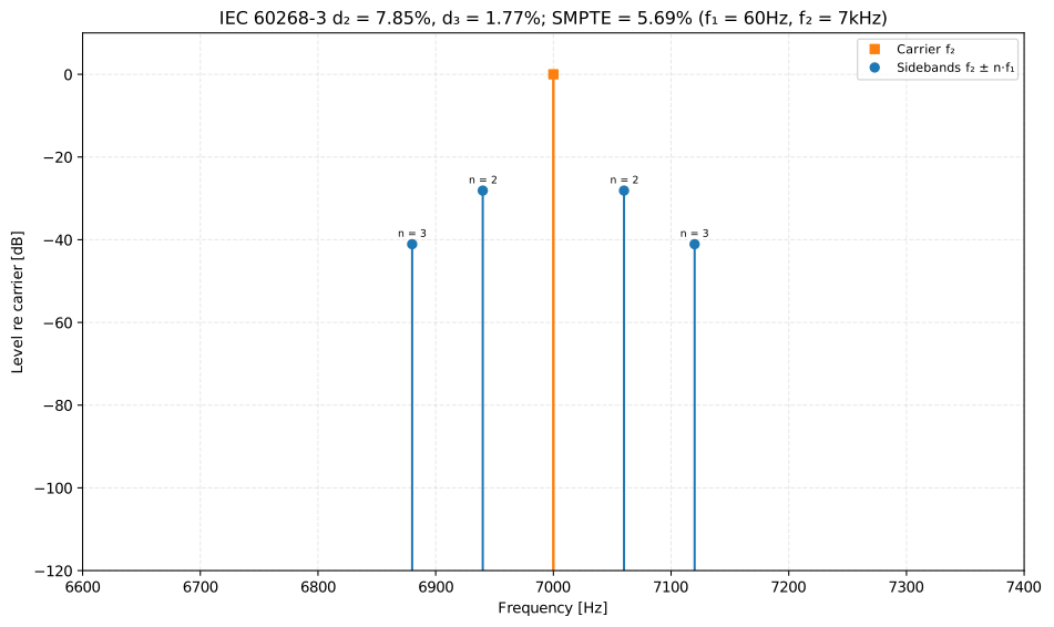
The ModulationDistortionResult is plottable: .plot() draws the output amplitude at the carrier f₂ (the 0 dB reference) and the four modulation sidebands at f₂ ± f₁ and f₂ ± 2f₁, the modulation counterpart of the harmonic spectrum of section 1. The asymmetric ratio between the n = 2 and n = 3 pairs reads the balance between the quadratic and cubic terms of the non-linearity at a glance:

Show the code for this figure

import matplotlib.pyplot as plt
import numpy as np
from phonometry import electroacoustics

fs = 48000
t = np.arange(fs) / fs                        # 1 s -> tones land on FFT bins
x = np.sin(2 * np.pi * 60.0 * t) + 0.25 * np.sin(2 * np.pi * 7000.0 * t)
signal = x + 0.04 * x**2 + 0.012 * x**3       # weakly non-linear device output

md = electroacoustics.modulation_distortion(signal, fs, 60.0, 7000.0)
md.plot()
plt.show()

4. Frequency response and coherence (Bendat & Piersol)

Given an input x and the output y of a device, the frequency response H(f) is estimated from the Welch-averaged cross- and auto-spectra. Bendat & Piersol (Random Data, 4th ed.) give two estimators, differing in which channel carries the noise, plus the ordinary coherence γ², the fraction of the output power linearly explained by the input:

$$H_1=\frac{G_{xy}}{G_{xx}},H_2=\frac{G_{yy}}{G_{yx}},{\gamma }^2=\frac{|G_{xy}{|}^2}{G_{xx}{G}_{yy}}\in [0,1].$$

H1 is unbiased when the noise is on the output, H2 when it is on the input; for a noiseless linear path both recover the true response and γ² = 1. Additive output noise biases H2 upward and pulls the coherence down to SNR/(1+SNR).

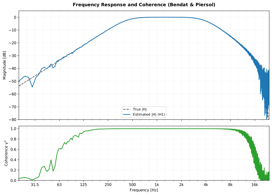
from phonometry import electroacoustics

res = electroacoustics.transfer_function(x, y, fs, estimator="H1")
print(res.magnitude_db, res.phase, res.coherence)
res.plot()   # Bode magnitude/phase + coherence (needs matplotlib)

freqs, gamma2 = electroacoustics.coherence(x, y, fs)

Coherence needs averaging over several Welch segments to be meaningful; a single segment gives γ² ≡ 1 by construction.

Show the code for this figure

import matplotlib.pyplot as plt
import numpy as np
from scipy import signal as sp
from phonometry import electroacoustics

fs = 48000
n = 400000
rng = np.random.default_rng(7)
x = rng.standard_normal(n)
b, a = sp.butter(2, [400.0, 4000.0], btype="band", fs=fs)   # device under test
y = sp.lfilter(b, a, x)
y = y + rng.standard_normal(n) * np.sqrt(np.mean(y ** 2)) * 0.05   # output noise

res = electroacoustics.transfer_function(x, y, fs, estimator="H1")
res.plot()
plt.show()

5. Sensitivity conventions (IEC 60268-4 / IEC 60268-5)

Distortion and response figures only compare across devices when the sensitivity conventions behind them match, and two conventions trip people constantly: the microphone reference level and the loudspeaker power-and-distance normalization.

Microphones (IEC 60268-4 clause 11). The sensitivity M is the output voltage per unit sound pressure, quoted in mV/Pa; the sensitivity level is LM = 20 lg(M / 1 V/Pa) dB, which is negative for every real microphone (a 50 mV/Pa studio condenser sits at −26 dB re 1 V/Pa). The classic pitfall is the reference: −26 dB re 1 V/Pa and +34 dB re 1 mV/Pa are the same microphone, 60 dB apart on paper, so a sensitivity level without its reference is meaningless. The standard also distinguishes free-field, diffuse-field and pressure sensitivity; for the same capsule they diverge at high frequency, so the stated type matters as much as the number.

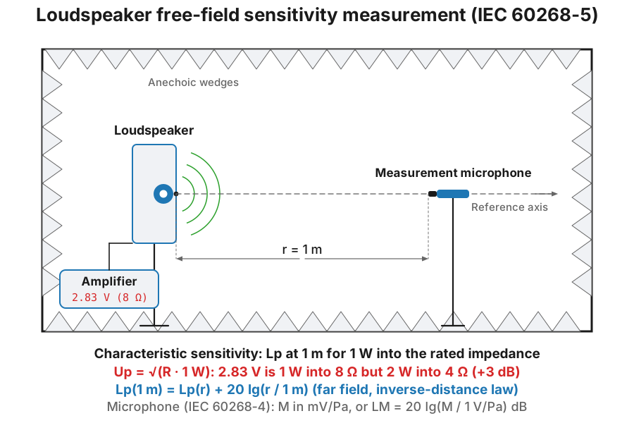
Loudspeakers (IEC 60268-5 clause 20.3). The characteristic sensitivity is the sound pressure produced at 1 m on the reference axis, in the free field, referred to an input of 1 W into the rated impedance; expressed as a level re 20 µPa (clause 20.4) it is the familiar “dB @ 1 W/1 m”. Two normalizations hide in that sentence:

• The electrical one. The test voltage is Up = √(R · 1 W), numerically √R: 2.83 V into a rated 8 Ω. A datasheet quoting “dB @ 2.83 V/1 m” for a 4 Ω loudspeaker is feeding it 2 W, which flatters the figure by 3 dB against a true 1 W/1 m rating; check the rated impedance before comparing.
• The geometric one. 1 m is a reference distance, not necessarily the measurement distance. The standard has you measure in the far field (at 0.5 m or an integer number of metres, clause 7.1) and refer the result back with the inverse-distance law, Lp(1 m) = Lp(r) + 20 lg(r / 1 m). That scaling only holds where the level actually falls 6 dB per doubling of distance, hence the free field of the diagram; at 1 m from a large multi-way cabinet the near field may not have ended yet, and the quoted “1 m” figure is then a referred quantity, not what a microphone placed at 1 m would read.

6. Radiating piston: radiation impedance and directivity

The rigid circular piston in an infinite baffle is the canonical radiator behind a loudspeaker cone, the open end of a duct and the radiation efficiency of any finite vibrating surface (Beranek & Mellow §4.19, §13.7). Its mechanical radiation impedance is $Z_r=\rho cS(R_1+j{X}_1)$ with $S=\pi a^2$ and the dimensionless resistance and reactance functions (Eqs. (13.117), (13.118))

$$R_1(x)=1-\frac{2J_1(x)}{x},X_1(x)=\frac{2H_1(x)}{x},x=2ka,$$

where $J_1$ is the Bessel function and $H_1$ the Struve function of order one. At low frequency $R_1\to (ka{)}^2/2$ and the reactance is mass-like with the radiation mass $M_r=8\rho a^3/3$ (Eq. (4.151)); at high frequency $R_1\to 1$, $X_1\to 0$ and the piston radiates as if into an infinite tube. The far field follows the directivity $D(\theta )=2J_1(ka\sin \theta )/(ka\sin \theta )$, whose first null is at $ka\sin \theta =3.8317$.

import numpy as np
from phonometry import radiating_piston

res = radiating_piston(radius=0.1, frequencies=np.geomspace(20, 20000, 200),
                       angles=np.linspace(0.0, np.pi / 2, 91))
print(round(res.radiation_mass, 4))            # 8 rho a^3 / 3, kg
print(round(float(res.directivity_index[0]), 2))  # 3.01 dB half-space limit
res.plot()                                      # R1 and X1 vs ka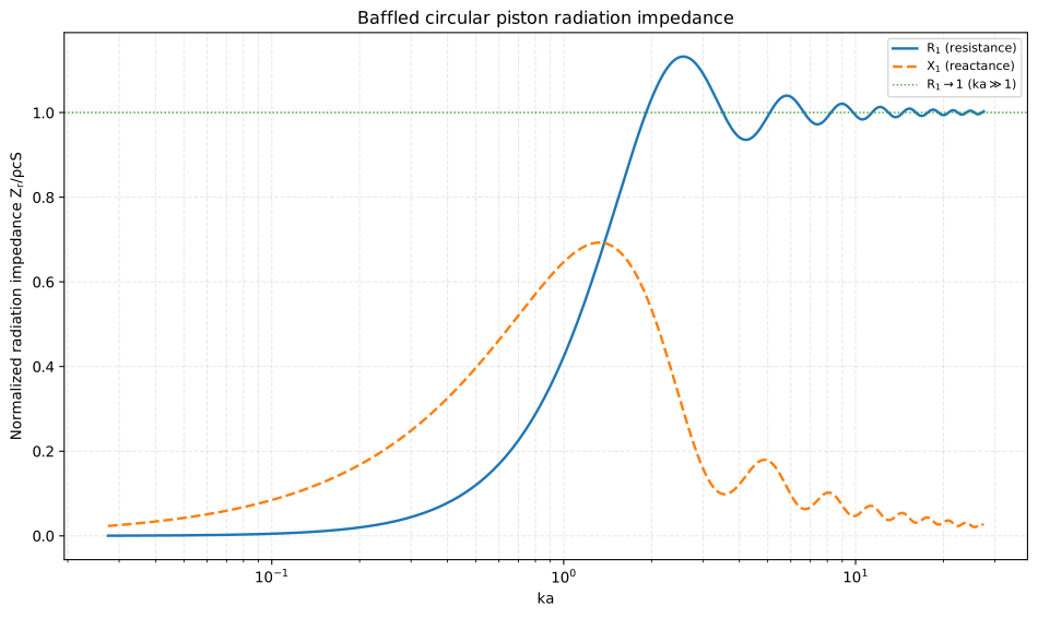

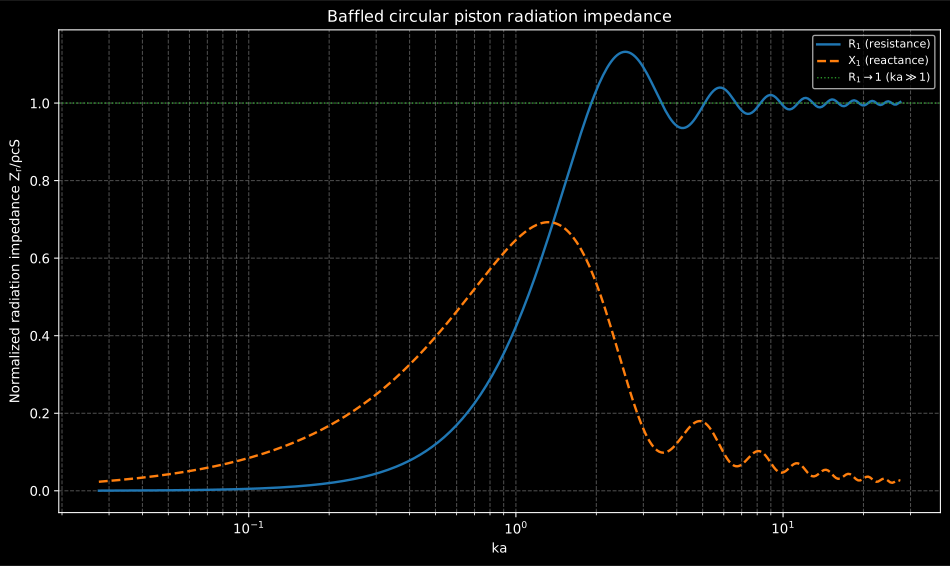
The .plot() of the result is the classic Beranek & Mellow impedance figure computed for this piston: below ka ≈ 1 the load is almost purely mass-like (X₁ dominates and R₁ ∝ (ka)², the regime where a loudspeaker’s output is stiffness- and mass-limited), and above it the resistance settles on ρcS with interference ripples while the reactance dies away.

Show the code for this figure

import matplotlib.pyplot as plt
import numpy as np
from phonometry import radiating_piston

res = radiating_piston(radius=0.075, frequencies=np.geomspace(20, 20000, 400))
res.plot()   # normalized R1 and X1 against ka
plt.show()

radiating_piston returns a RadiatingPistonResult with the normalized resistance/reactance, the mechanical radiation_resistance/radiation_reactance, the radiation_mass, the directivity_index, the far-field directivity pattern (when angles are given) and .plot(). The building blocks piston_resistance, piston_reactance and piston_directivity are also callable directly. The piston is the companion radiator model of the industrial noise-control silencers.

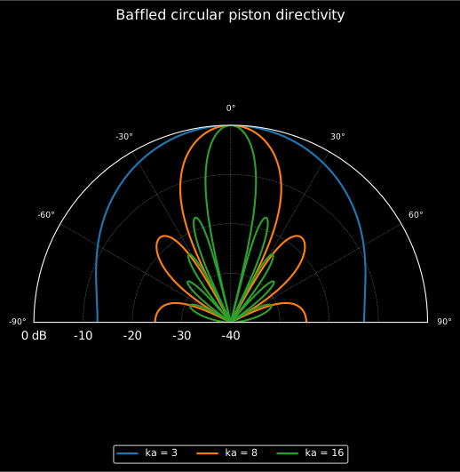
The directivity pattern itself is a plottable result of its own: piston_directivity_pattern(ka) samples $D(\theta )$ at one or more $ka$ values and returns a PistonDirectivity (the polar angle grid, the linear directivity and its dB form directivity_db, and the ka values) whose .plot() draws the classic beam pattern. Several $ka$ are shown as one family on the same polar axes, so the narrowing of the main lobe and the emergence of the side lobes read at a glance:

from phonometry import piston_directivity_pattern

pattern = piston_directivity_pattern([3.0, 8.0, 16.0])
print(pattern.directivity_db.shape)  # (3, 361): one row per ka
pattern.plot()                       # polar beam pattern in dB (needs matplotlib)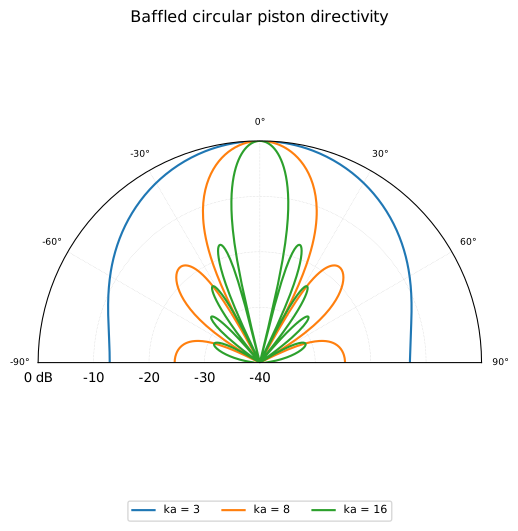

Show the code for this figure

import matplotlib.pyplot as plt
from phonometry import piston_directivity_pattern

piston_directivity_pattern([3.0, 8.0, 16.0]).plot()
plt.show()

7. Loudspeaker characteristics report (IEC 60268-5)

The rated characteristics IEC 60268-5 defines around a measured on-axis response gather into a single loudspeaker characteristics result that renders the standard’s rated-characteristics data sheet. Two of the numbers are computed from the response rather than merely repeated:

• Characteristic sensitivity level (20.3/20.4). The on-axis level averaged over a stated band, referred to 1 W into the rated impedance $R$ at 1 m: $L_M=\overline{L}+20\lg (d/d_0)+20\lg (U_p/U)$ with $U_p=\sqrt{R\cdot 1\text{W}}=\sqrt{R}$. The default drive is that $\sqrt{R}$ (2.83 V into 8 Ω), so with a 1 m response the sensitivity level is the band mean.
• Effective frequency range (21.2). The band over which the response stays within 10 dB of the level averaged over the one-octave band in the region of maximum sensitivity; troughs narrower than 1/9 octave are neglected.

import numpy as np
from phonometry import loudspeaker_characteristics, radiating_piston, ReportMetadata

freqs = np.geomspace(30, 24000, 320)
spl = 87.0 + 1.2 * np.sin(2 * np.log2(freqs / 900.0))
spl -= 10 * np.log10(1 + (50.0 / freqs) ** 6)       # low-frequency roll-off
spl -= 10 * np.log10(1 + (freqs / 16000.0) ** 7)    # high-frequency roll-off

result = loudspeaker_characteristics(
    freqs, spl, rated_impedance=8.0, sensitivity_band=(200.0, 4000.0),
    impedance=(np.geomspace(20, 20000, 260),
               6.6 + 24 * np.exp(-(np.log2(np.geomspace(20, 20000, 260) / 52.0) ** 2) / 0.12)),
    distortion=(np.geomspace(50, 5000, 140),
                0.3 + 2.6 * np.exp(-(np.log2(np.geomspace(50, 5000, 140) / 70.0) ** 2) / 0.45)),
    directivity=radiating_piston(0.075, np.array([1000.0, 2000.0, 4000.0]),
                                 angles=np.radians(np.linspace(0, 90, 46))),
    polar_frequency=2000.0,
)
print(round(result.sensitivity_level_db, 1))                 # dB, 1 W / 1 m
print(tuple(round(x) for x in result.effective_range))       # Hz

result.report("loudspeaker.pdf", metadata=ReportMetadata(measurement_standard="IEC 60268-5"))

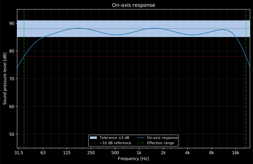
loudspeaker_characteristics returns a LoudspeakerCharacteristics with the computed sensitivity_level_db, effective_range, reference_level_db, characteristic_sensitivity_pa and minimum_impedance, and a .report() that writes the fiche. The on-axis response is drawn with its tolerance band and the effective-range markers to the IEC 60263 proportion (one frequency decade equal to 25 dB), and the polar directivity on the IEC 60263 25 dB reference circle. 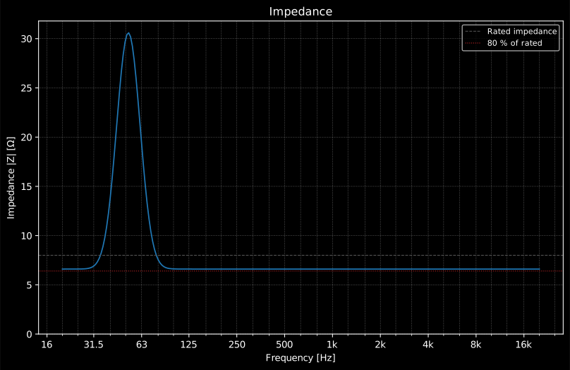The impedance modulus (with the 80 %-of-rated line), the total-harmonic-distortion curve and the directivity feed the secondary panels, reusing the radiating piston directivity of section 6 and a swept-sine THD result for the distortion curve.

The rated characteristics are also available interactively through .plot(), which draws one concept per figure with the same panel code the report composes, selected by quantity. Passing an axes draws on it:

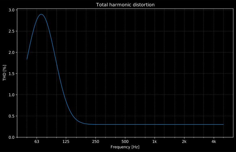
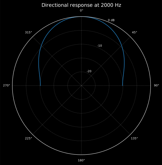
result.plot()                        # on-axis response (default)
result.plot(quantity="impedance")    # |Z| modulus with the rated / 80 % lines
result.plot(quantity="thd")          # total harmonic distortion vs frequency
result.plot(quantity="directivity")  # polar response on the 25 dB circle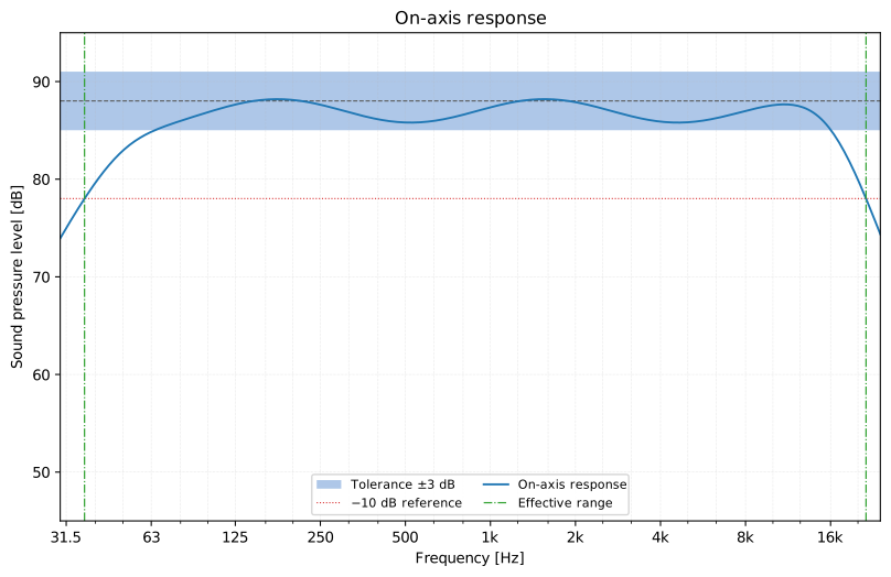

Show the code for this figure

import matplotlib.pyplot as plt
import numpy as np
from phonometry import loudspeaker_characteristics

freqs = np.geomspace(30, 24000, 320)
spl = 87.0 + 1.2 * np.sin(2 * np.log2(freqs / 900.0))
spl -= 10 * np.log10(1 + (50.0 / freqs) ** 6)       # low-frequency roll-off
spl -= 10 * np.log10(1 + (freqs / 16000.0) ** 7)    # high-frequency roll-off

result = loudspeaker_characteristics(freqs, spl, rated_impedance=8.0,
                                     sensitivity_band=(200.0, 4000.0))
result.plot()   # quantity="response" (the default)
plt.show()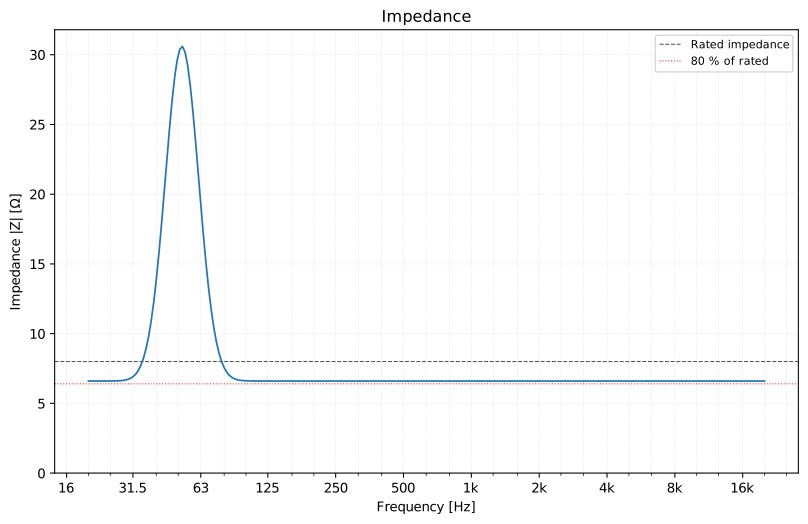

Show the code for this figure

import matplotlib.pyplot as plt
import numpy as np
from phonometry import loudspeaker_characteristics

freqs = np.geomspace(30, 24000, 320)
spl = 87.0 - 10 * np.log10(1 + (50.0 / freqs) ** 6)
fz = np.geomspace(20, 20000, 260)

result = loudspeaker_characteristics(
    freqs, spl, rated_impedance=8.0, sensitivity_band=(200.0, 4000.0),
    impedance=(fz, 6.6 + 24 * np.exp(-(np.log2(fz / 52.0) ** 2) / 0.12)),
)
result.plot(quantity="impedance")
plt.show()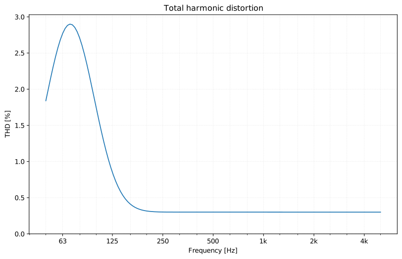

Show the code for this figure

import matplotlib.pyplot as plt
import numpy as np
from phonometry import loudspeaker_characteristics

freqs = np.geomspace(30, 24000, 320)
spl = 87.0 - 10 * np.log10(1 + (50.0 / freqs) ** 6)
thd_f = np.geomspace(50, 5000, 140)

result = loudspeaker_characteristics(
    freqs, spl, rated_impedance=8.0, sensitivity_band=(200.0, 4000.0),
    distortion=(thd_f, 0.3 + 2.6 * np.exp(-(np.log2(thd_f / 70.0) ** 2) / 0.45)),
)
result.plot(quantity="thd")
plt.show()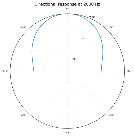

Show the code for this figure

import matplotlib.pyplot as plt
import numpy as np
from phonometry import loudspeaker_characteristics, radiating_piston

freqs = np.geomspace(30, 24000, 320)
spl = 87.0 - 10 * np.log10(1 + (50.0 / freqs) ** 6)

result = loudspeaker_characteristics(
    freqs, spl, rated_impedance=8.0, sensitivity_band=(200.0, 4000.0),
    directivity=radiating_piston(0.075, np.array([1000.0, 2000.0, 4000.0]),
                                 angles=np.radians(np.linspace(0, 90, 46))),
    polar_frequency=2000.0,
)
result.plot(quantity="directivity")
plt.show()

The example fiche is regenerated with make reports and kept rendered in the repository; click the preview to open the PDF.

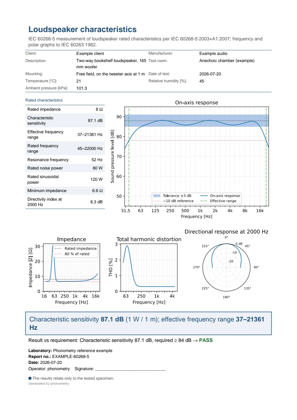
One-page IEC 60268-5 loudspeaker rated-characteristics fiche: a header with the manufacturer and model, the rated-characteristics table (rated impedance, characteristic sensitivity, effective and rated frequency ranges, resonance frequency, rated powers, minimum impedance and directivity index) beside the on-axis frequency response with its tolerance band and effective-range markers, and the impedance, total-harmonic-distortion and polar-directivity panels, all drawn to the IEC 60263 scale conventions.

Download the report (PDF)

Loudspeaker characteristics fiche (LoudspeakerCharacteristics.report), the IEC 60268-5 rated-characteristics table beside the on-axis response, impedance, THD and polar panels drawn to the IEC 60263 25 dB-per-decade and 25 dB reference-circle conventions.

8. Microphone characteristics report (IEC 60268-4)

The microphone companion of section 7: the rated characteristics IEC 60268-4 defines around a measured free-field frequency response gather into a single microphone characteristics result that renders the standard’s rated-characteristics data sheet. Four of the numbers are computed from the standard’s own definitions rather than merely repeated:

• Sensitivity level (11.1). The rated free-field sensitivity $M$ (mV/Pa, at the 1 kHz reference frequency of 11.3) as a level, $L_M=20\lg (M/1\text{V/Pa})$: 12.5 mV/Pa is $-38.1$ dB re 1 V/Pa.
• Effective frequency range (12.2). The band over which the response, normalized to 0 dB at the reference frequency, stays within the stated $\pm$ tolerance; the edges are the interpolated tolerance crossings.
• Directivity index (13.2.2). $D=20\lg (M_0/M_{\mathrm{diff}})$ with the diffuse-field sensitivity from the 11.2.2 a) integral over a rotationally symmetric pattern; the ideal cardioid returns $10\lg 3=4.8$ dB.
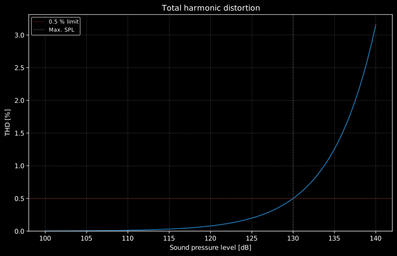
• Equivalent noise level (17.2). The weighted inherent-noise voltage over the rated sensitivity as a sound pressure level, $L_N=20\lg ((U_N/M)/20\mu \text{Pa})$, with the signal-to-noise ratio re 1 Pa (94 dB SPL) derived from it. The overload sound pressure level (15.2) is read from a distortion-against-level curve at the stated THD limit.

import numpy as np
from phonometry import microphone_characteristics, ReportMetadata

freqs = np.geomspace(20, 20000, 400)
response = -10 * np.log10(1 + (30.0 / freqs) ** 4)      # low-frequency roll-off
response -= 10 * np.log10(1 + (freqs / 19000.0) ** 8)   # high-frequency roll-off
response += 2.0 * np.exp(-(np.log2(freqs / 9000.0) ** 2) / 0.3)  # presence region

angles = np.linspace(0, 179, 359)
cardioid = 20 * np.log10((1 + np.cos(np.radians(angles))) / 2)

result = microphone_characteristics(
    freqs, response, 12.5, tolerance_db=3.0,          # 12.5 mV/Pa at 1 kHz
    rated_impedance=150.0, minimum_load_impedance=1000.0,
    noise_voltage=1.25e-6,                             # A-weighted, V
    max_spl_thd_percent=0.5,
    distortion=(np.linspace(100, 140, 81),
                0.5 * 10 ** ((np.linspace(100, 140, 81) - 130.0) * 0.08)),
    polar=(angles, cardioid), polar_frequency=1000.0,
    powering="Phantom P48 (IEC 61938)", supply_current_ma=3.1,
)
print(round(result.sensitivity_level_db, 1))            # -38.1 dB re 1 V/Pa
print(tuple(round(x) for x in result.effective_range))  # Hz
print(round(result.directivity_index_db, 1))            # 4.8 dB (cardioid)
print(round(result.equivalent_noise_level_db, 1))       # dB(A)

result.report("microphone.pdf", metadata=ReportMetadata(measurement_standard="IEC 60268-4"))

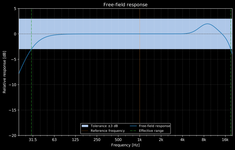
microphone_characteristics returns a MicrophoneCharacteristics with the computed sensitivity_level_db, effective_range, directivity_index_db, equivalent_noise_level_db, max_spl_db, signal_to_noise_ratio_db and diffuse_field_sensitivity_level_db, and a .report() that writes the fiche. The free-field response is drawn with its tolerance band, the reference-frequency marker and the effective-range markers to the IEC 60263 proportion (one frequency decade equal to 25 dB), and the directional pattern on the IEC 60263 25 dB reference circle; the inherent-noise spectrum and the distortion-against-level curve (with the THD limit and the overload level marked) feed the secondary panels. A requirement in the metadata is checked as a maximum permitted equivalent noise level.

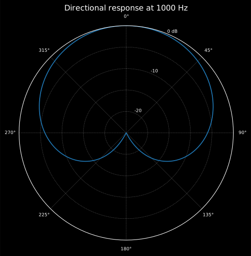
The rated characteristics are also available interactively through .plot(), which draws one concept per figure with the same panel code the report composes, selected by quantity. Passing an axes draws on it:

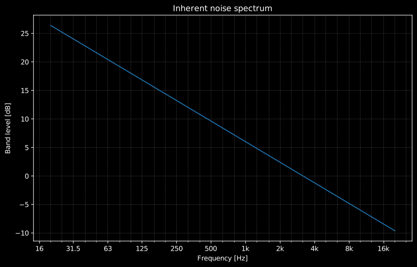
result.plot()                        # free-field response (default)
result.plot(quantity="directivity")  # polar pattern on the 25 dB circle
result.plot(quantity="noise")        # inherent-noise band spectrum
result.plot(quantity="distortion")   # THD vs sound pressure level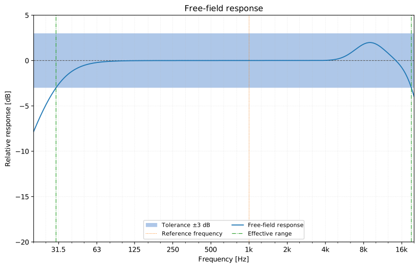

Show the code for this figure

import matplotlib.pyplot as plt
import numpy as np
from phonometry import microphone_characteristics

freqs = np.geomspace(20, 20000, 400)
response = -10 * np.log10(1 + (30.0 / freqs) ** 4)      # low-frequency roll-off
response -= 10 * np.log10(1 + (freqs / 19000.0) ** 8)   # high-frequency roll-off
response += 2.0 * np.exp(-(np.log2(freqs / 9000.0) ** 2) / 0.3)  # presence region

result = microphone_characteristics(freqs, response, 12.5, tolerance_db=3.0)
result.plot()   # quantity="response" (the default)
plt.show()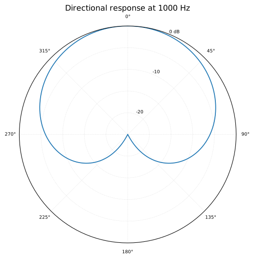

Show the code for this figure

import matplotlib.pyplot as plt
import numpy as np
from phonometry import microphone_characteristics

freqs = np.geomspace(20, 20000, 400)
response = -10 * np.log10(1 + (30.0 / freqs) ** 4)
angles = np.linspace(0, 179, 359)
cardioid = 20 * np.log10((1 + np.cos(np.radians(angles))) / 2)

result = microphone_characteristics(
    freqs, response, 12.5, tolerance_db=3.0,
    polar=(angles, cardioid), polar_frequency=1000.0,
)
result.plot(quantity="directivity")
plt.show()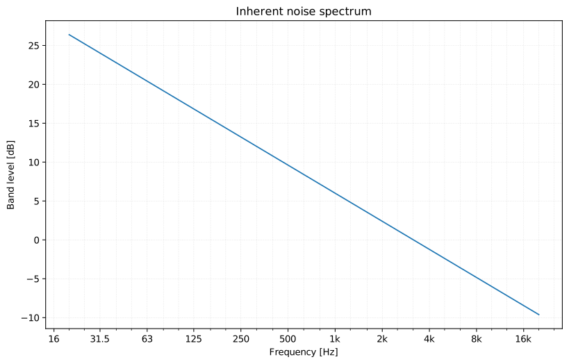

Show the code for this figure

import matplotlib.pyplot as plt
import numpy as np
from phonometry import microphone_characteristics

freqs = np.geomspace(20, 20000, 400)
response = -10 * np.log10(1 + (30.0 / freqs) ** 4)
noise_f = np.geomspace(20, 20000, 31)

result = microphone_characteristics(
    freqs, response, 12.5, tolerance_db=3.0, noise_voltage=1.25e-6,
    noise_spectrum=(noise_f, 6.0 + 12.0 * np.log10(1000.0 / noise_f)),
)
result.plot(quantity="noise")
plt.show()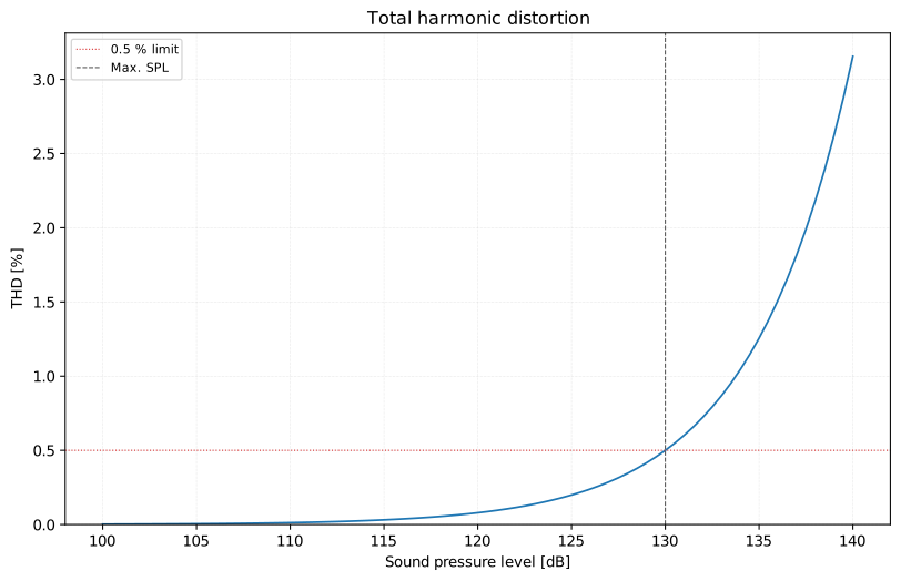

Show the code for this figure

import matplotlib.pyplot as plt
import numpy as np
from phonometry import microphone_characteristics

freqs = np.geomspace(20, 20000, 400)
response = -10 * np.log10(1 + (30.0 / freqs) ** 4)
spl_axis = np.linspace(100, 140, 81)

result = microphone_characteristics(
    freqs, response, 12.5, tolerance_db=3.0, max_spl_thd_percent=0.5,
    distortion=(spl_axis, 0.5 * 10 ** ((spl_axis - 130.0) * 0.08)),
)
result.plot(quantity="distortion")
plt.show()

The example fiche is regenerated with make reports and kept rendered in the repository; click the preview to open the PDF.

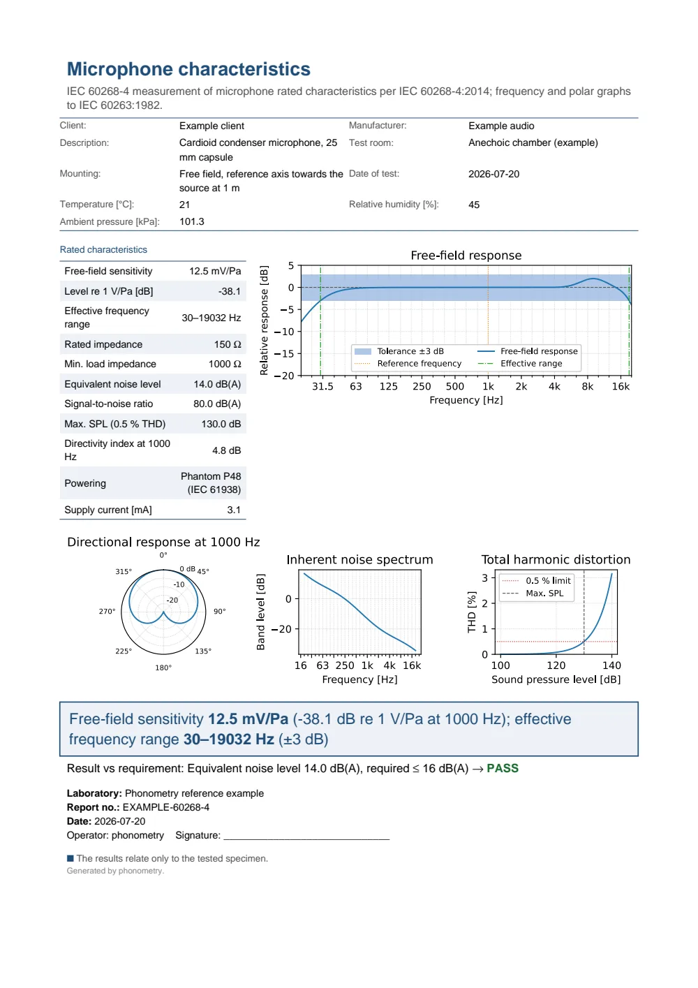
One-page IEC 60268-4 microphone rated-characteristics fiche: a header with the manufacturer and model, the rated-characteristics table (free-field sensitivity in mV/Pa and its level re 1 V/Pa, effective frequency range, rated and minimum load impedances, equivalent noise level, signal-to-noise ratio, maximum SPL at the stated THD limit, directivity index and phantom powering) beside the free-field frequency response with its tolerance band and effective-range markers, and the directional-pattern, inherent-noise-spectrum and distortion panels, all drawn to the IEC 60263 scale conventions.

Download the report (PDF)

Microphone characteristics fiche (MicrophoneCharacteristics.report), the IEC 60268-4 rated-characteristics table beside the free-field response, with the cardioid directional pattern, inherent-noise and THD-against-level panels drawn to the IEC 60263 25 dB-per-decade and 25 dB reference-circle conventions.

What this guide covers

Covered. The IEC 60268-3 distortion set (clauses 14.12.2-14.12.11): THD_F and THD_R (thd), nth-order harmonic distortion (harmonic_distortion), THD+N and SINAD through the AES17-2015 measurement bandwidth (harmonic_analysis, AES17 clauses 5.2.5/5.2.8/6.3.1), modulation and difference-frequency intermodulation, dynamic intermodulation (DIM) and the ITU-R BS.468-4 weighted THD, plus the AES17-2015 dynamic range and idle channel noise. The Bendat & Piersol H1/H2 frequency-response estimators and ordinary coherence. The IEC 60268-4:2014 microphone rated characteristics (sensitivity, frequency response and range, directivity index, overload SPL, equivalent noise level, impedances and power) via microphone_characteristics and its .report(). The IEC 60268-5:2003+A1:2007 loudspeaker rated characteristics (sensitivity, frequency range, directivity index, THD against frequency) via loudspeaker_characteristics and its .report(), both drawn to the IEC 60263 scale conventions. The baffled-piston radiation model (radiating_piston, Beranek & Mellow §4.19/§13.7).

Not covered. Other parts of the IEC 60268 series sit outside this page: Part 16 (objective speech intelligibility, the speech transmission index) is not implemented. The implemented editions are frozen at IEC 60268-4:2014, IEC 60268-5:2003+A1:2007 and AES17-2015; the superseding IEC 60268-4:2018 and AES17-2020 revisions are not the ones checked.

See also

• Industrial noise control: reactive silencers, HVAC duct methods and machine enclosures, sharing the radiating piston as the canonical radiator.
• Swept-sine distortion: the Farina/Novak harmonic separation whose THD(f) feeds the loudspeaker distortion panel.
• API reference: electroacoustics.distortion, electroacoustics.frequency_response, electroacoustics.piston, electroacoustics.loudspeaker and electroacoustics.microphone.

References

• Audio Engineering Society. (2015). AES standard method for digital audio engineering — Measurement of digital audio equipment (AES17-2015). Clauses 5.2.5, 5.2.8 and 6.3.1: the THD+N ratio via the standard notch filter and the standard measurement bandwidth; SINAD is derived from it. Since revised as AES17-2020 (same catalogue page); the 2015 edition is the implemented one.
• Bendat, J. S., & Piersol, A. G. (2010). Random data: Analysis and measurement procedures (4th ed.). Wiley. https://doi.org/10.1002/9781118032428ISBN 978-0-470-24877-5. The H1 and H2 frequency-response estimators and the ordinary coherence γ² of section 4.
• Beranek, L. L., & Mellow, T. J. (2012). Acoustics: Sound fields and transducers. Academic Press. https://doi.org/10.1016/C2011-0-05897-0ISBN 978-0-12-391421-7. The transducer physics behind section 5: loudspeaker radiation, on-axis pressure and the near-field to far-field transition.
• International Electrotechnical Commission. (1982). Scales and sizes for plotting frequency characteristics and polar diagrams (IEC 60263:1982). The scale proportions of the section 7 characteristic graphs: one frequency decade equal to 25 dB on the ordinate (clause 2), and the polar diagram plotted on a 25 dB reference-circle radius (clause 3).
• International Electrotechnical Commission. (2003). Sound system equipment – Part 5: Loudspeakers (IEC 60268-5:2003+A1:2007). The rated loudspeaker characteristics of section 7: the rated impedance (16), the rated frequency range (19.1), the characteristic sensitivity and its level referred to 1 W at 1 m (20.3/20.4), the effective frequency range against the -10 dB band (21.2), the directivity index (23.3) and the total harmonic distortion against frequency (24.1).
• International Electrotechnical Commission. (2013). Sound system equipment – Part 3: Amplifiers (IEC 60268-3:2013). Clauses 14.12.2-14.12.11: total harmonic distortion THD_F/THD_R (the 14.12.3.2 formula defines the R form), nth-order harmonic distortion d_n, the per-order modulation (d_m,n) and difference-frequency (d_d,n) intermodulation, total difference-frequency distortion, dynamic intermodulation (DIM) and the ITU-R BS.468-4 / IEC 60268-1 weighted THD.
• International Electrotechnical Commission. (2014). Sound system equipment – Part 4: Microphones (IEC 60268-4:2014). The rated microphone characteristics of sections 5 and 8: the free-field sensitivity and its level re 1 V/Pa (11.1/11.3), the frequency response and effective frequency range (12.1/12.2), the directional pattern and the directivity index through the 11.2.2 a) diffuse-field integral (13.1/13.2), the overload sound pressure level (15.2), the equivalent sound pressure level due to inherent noise (17) and the rated impedances and power supply (9/10). Since revised as IEC 60268-4:2018 (same catalogue page); the 2014 edition is the implemented one.
• International Telecommunication Union. (1986). Measurement of audio-frequency noise voltage level in sound broadcasting (Recommendation ITU-R BS.468-4). The weighting-network nominal response behind the weighted THD (the IEC 60268-1 Appendix A curve).