Structure-borne sound power of equipment (EN 15657)

Building service equipment (pumps, fans, boilers, sanitary appliances) injects structure-borne sound power into the building structure it is fixed to, which then re-radiates as airborne noise in adjoining rooms. EN 15657:2018 measures it with the reception-plate method: the source is mounted on a plate of known mass per unit area m and area S whose structural loss factor η is known, and the plate’s spatial-average vibratory velocity is measured. Formula (14) gives the power injected into that particular plate; the plate-independent source quantities (the equivalent blocked force, Formula 15; the characteristic reception-plate power level L_Wsn, Formula 17; and the equivalent free velocity and source mobility, Formulae 18/19) are derived from it and are what the EN 12354-5 installed-equipment prediction consumes.

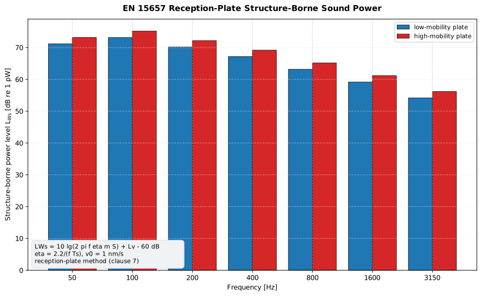
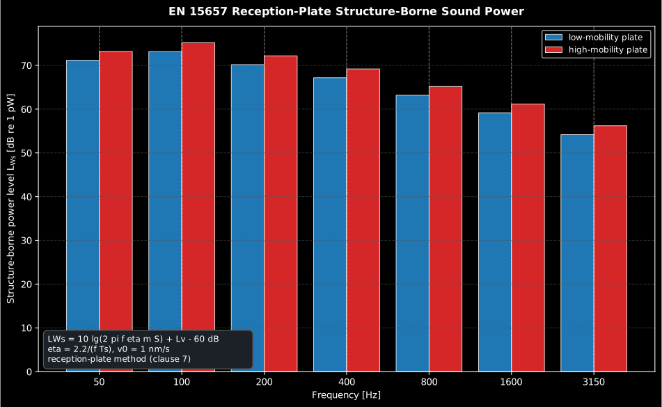
Show the code for this figure

import matplotlib.pyplot as plt
import numpy as np
from phonometry import building

# The same pump-like source measured on a heavy and on a light reception plate.
bands = np.array([50.0, 100.0, 200.0, 400.0, 800.0, 1600.0, 3150.0])
lv_low = np.array([88.0, 90.0, 87.0, 84.0, 80.0, 76.0, 71.0])

low = building.reception_plate_power(lv_low, bands, mass_per_area=600.0,
                                     area=2.0, reverberation_time=0.8)
high = building.reception_plate_power(lv_low + 6.0, bands, mass_per_area=150.0,
                                      area=2.0, reverberation_time=0.5)

# One line — the L_Ws(f) bars of one determination with its band-summed total:
low.plot()
plt.show()

# By hand, comparing the two plates from the results' fields:
x = np.arange(bands.size)
fig, ax = plt.subplots()
ax.bar(x - 0.2, low.power_level, width=0.4, label="low-mobility plate")
ax.bar(x + 0.2, high.power_level, width=0.4, label="high-mobility plate")
ax.set_xticks(x, [f"{b:g}" for b in bands])
ax.set(xlabel="Frequency [Hz]",
       ylabel="Structure-borne power level $L_{Ws}$ [dB re 1 pW]")
ax.legend()
plt.show()

1. The reception-plate relations

Why a plate at all? Characterising the source by its contact forces directly would mean instrumenting every fixing point in up to six components each (three forces, three moments), on a machine that must keep running normally. The reception plate sidesteps the whole contact problem: let the source run on a resonant plate whose dissipation is known, wait for the steady state, and then the power the plate dissipates equals the power the source injects, over all contacts and components at once. One spatial average of the plate velocity replaces the entire force-measurement problem.

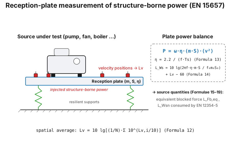
The power a resonant plate dissipates is P = ω·η·(m·S)·⟨v²⟩, so the injected power level in one-third-octave bands is (Formula 14)

$$L_{Ws}=10\lg \left(\frac{2\pi f\eta mS}{f_0{m}_0{S}_0}\right)+L_v-60[\mathrm{dB}\mathrm{re}1\mathrm{pW}],$$

with references f₀ = 1 Hz, m₀ = 1 kg, S₀ = 1 m²; the −60 dB term is 10 lg(v₀²/P₀) for the EN 15657 velocity reference v₀ = 10⁻⁹ m/s. The plate velocity is the energetic spatial average over the N positions (Formula 12) and the loss factor comes from the structural reverberation time Ts (Formula 13, identical to the ISO 10848 total loss factor):

$$L_v=10\lg (\frac{1}{N}\sum 10^{L_{v,i}/10}),\eta =\frac{2.2}{f{T}_s}.$$

import numpy as np
from phonometry import building

bands = np.array([100.0, 200.0, 400.0, 800.0])
lv_i = np.array([88.0, 90.0, 87.0, 89.0, 86.0, 90.0])   # six plate positions @ 200 Hz
print(round(building.spatial_mean_velocity_level(lv_i), 2))    # 88.6 dB re 1 nm/s

# Power level injected into the reception plate (loss factor from Ts):
res = building.reception_plate_power(
    velocity_level=np.array([90.0, 87.0, 82.0, 77.0]),
    frequency=bands, mass_per_area=600.0, area=2.0, reverberation_time=0.8,
)
print(np.round(res.power_level, 1))     # per-band L_Ws
print(round(res.total_level, 1))        # band-summed level [dB re 1 pW]

res.plot()   # the L_Ws(f) bars with the band-summed total, as in the figure above (needs matplotlib)

2. Low- and high-mobility plates

Two reception plates bracket the installation conditions. On the low-mobility (heavy) plate the source’s own dynamics barely change the plate’s point mobility or loss factor; the high-mobility (light) plate is dynamically loaded by the source, so its reverberation time and mobility are measured with the source attached. The plate-injected power plus the plate’s point mobility (see mechanical mobility) yield the source description for the EN 12354-5 model through the conversion chain below.

3. From plate power to source quantities (Formulae 15–19)

The plate-injected L_Ws is not a source descriptor: the same source injects a different power into a different receiver. EN 15657 derives the plate-independent quantities: the equivalent blocked force level (Formula 15, re F₀ = 10⁻⁶ N) from the low-mobility plate,

$$L_{Fb,eq}=L_{Ws,\mathrm{low}}-10\lg \frac{\mathrm{Re}\{Y_{R,\mathrm{low},\mathrm{eq}}\}}{Y_0},$$

the characteristic reception-plate power level that EN 12354-5 consumes (Formula 17), referred to the standard 10 cm concrete plate of characteristic mobility Y_R,∞,low = 5·10⁻⁶ m/(N·s) (clause 7.2.4),

$$L_{Wsn}=L_{Fb,eq}+10\lg \frac{Y_{R,\infty ,\mathrm{low}}}{Y_0},$$

and, from the high-mobility plate, the equivalent free velocity level (Formula 18, re 10⁻⁹ m/s) and the source mobility |Y_S,eq| (Formula 19). The EN 12354-5 Annex I mobility correction (installed_power_from_reception_plate, see installed structure-borne sound) then refers L_Wsn to the actual receiving element.

from phonometry import building

# EN 12354-5 Annex I.3 (flushing cistern, wall contact, 63 Hz): measured on a
# plate of Y = 5.34e-6 m/(N·s); the wall's characteristic mobility is 24.1e-6.
lfb = building.equivalent_blocked_force_level(61.7, 5.34e-6)      # Formula (15)
lwsn = building.characteristic_reception_plate_power(lfb)         # Formula (17)
inst = building.installed_power_from_reception_plate(lwsn, 24.1e-6)  # Annex I
print(round(float(lwsn), 1), round(float(inst), 1))         # 61.4 68.2  (Table I.8)

# Free velocity (Formula 18) + blocked force close the source mobility (19):
lvf = building.equivalent_free_velocity_level(70.0, 1.0e-2)
print(float(building.source_mobility_from_levels(lvf, lfb)))      # |Y_S,eq| in m/(N·s)

The direct source-side counterpart is the ISO 9611 free velocity level (re v₀ = 5·10⁻⁸ m/s) measured at the contact points of resiliently mounted machinery; its equation (9) position average is mean_free_velocity_level().

4. The characterization report (.report())

A characterization ends as a document. The StructureBornePowerResult exposes a .report() method that writes a one-page PDF fiche laid out like a sound-power test sheet: the standard-basis line naming the EN 15657:2018 reception-plate method (Formula 14), an optional metadata header (client, source equipment, test environment, instrumentation, climate, date), a per-band table (nominal octave/one-third-octave frequency, the spatial mean plate velocity level $L_v$ and the injected structure-borne sound power level $L_{Ws}$), the $L_{Ws}(f)$ spectrum with a nominal band axis, and a boxed band-summed total $L_{Ws}$ (dB re 1 pW) with the plate mass per area $m$ and area $S$.

The metadata is supplied through a ReportMetadata, whose applicable fields here are the source equipment (specimen), the test environment (test_room), the client, the instrumentation, the temperature, relative humidity and ambient pressure, the date of test (test_date) and the footer identity (laboratory, operator, report_id, notes); the plate mass and area come from the result itself. Supplying requirement adds a PASS/FAIL verdict against a declared upper limit on the total $L_{Ws}$ (a power emission is a quantity where less is better, so the source passes at or below the limit). verbose=True adds the plate loss factor $\eta$ column to the table. language="es" renders the Spanish fiche with comma decimals. The basis strip states Formula 14 and reminds that the plate-injected level must be converted to the plate-independent source quantities (Formulae 15/17) before it feeds EN 12354-5.

import numpy as np
from phonometry import ReportMetadata, reception_plate_power

freqs = np.array([125, 250, 500, 1000, 2000, 4000], float)
lv = np.array([88.0, 90, 86, 82, 78, 73])   # spatial mean plate velocity level [dB]
res = reception_plate_power(
    lv, freqs, mass_per_area=25.0, area=1.2, reverberation_time=0.3,
)

res.report(
    "structure_borne_power.pdf",
    metadata=ReportMetadata(
        client="Example building services contractor",
        specimen="Circulation pump (wall-mounted)",
        test_room="Reception-plate test rig (heavy concrete plate)",
        laboratory="Phonometry reference example",
        report_id="EXAMPLE-15657",
    ),
)   # total L_Ws ~ 65 dB re 1 pW

The example fiche is regenerated with make reports and kept rendered in the repository; click the preview to open the PDF.

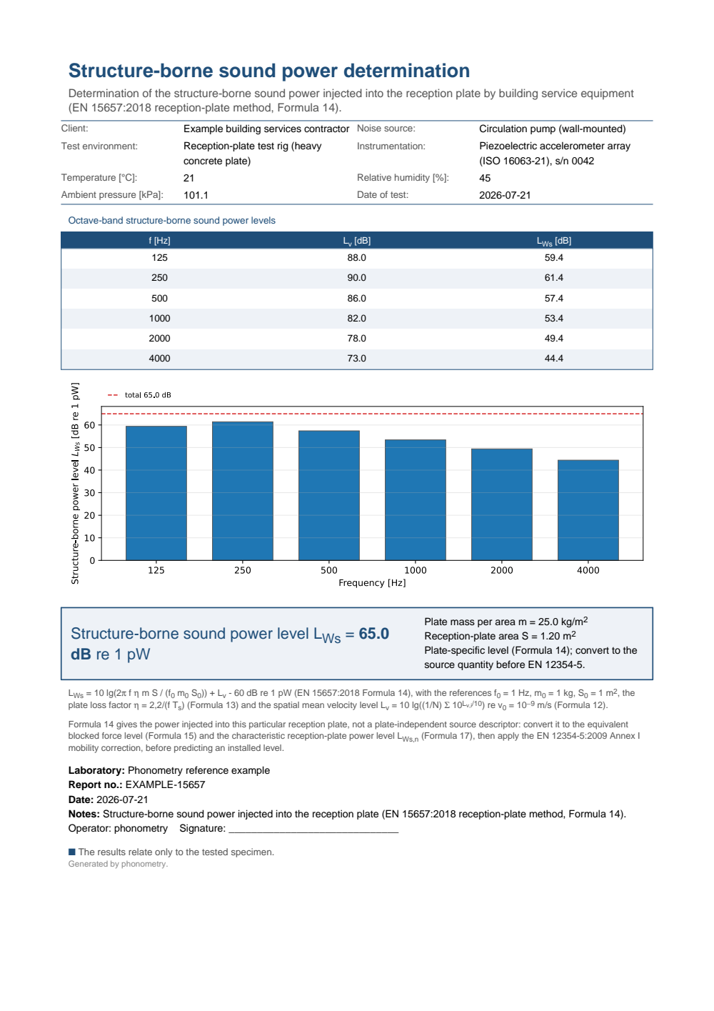
One-page EN 15657:2018 reception-plate structure-borne sound power fiche: a header with the client, the source equipment, the reception-plate test rig and the accelerometer and climate, the octave-band table (125 Hz to 4 kHz) of spatial mean plate velocity levels Lv and injected structure-borne sound power levels L_Ws, the L_Ws(f) spectrum with a nominal band axis, and the boxed band-summed total L_Ws (dB re 1 pW) with the plate mass per area m = 25 kg/m2 and area S = 1.20 m2, closed by a basis strip stating the Formula 14 relation and the conversion to the plate-independent source quantities required before EN 12354-5.

Download the report (PDF)

Structure-borne sound power fiche (StructureBornePowerResult.report), an EN 15657 reception-plate characterization with the boxed total L_Ws.

What this guide covers

Covered. EN 15657:2018’s reception-plate method: the spatial mean velocity level (spatial_mean_velocity_level, Formula 12), the plate loss factor (plate_loss_factor, Formula 13) and the plate-injected power level (reception_plate_power, structure_borne_power_level, Formula 14). Also the plate-independent source-quantity chain: the equivalent blocked force level (equivalent_blocked_force_level, Formula 15), the characteristic reception-plate power level (characteristic_reception_plate_power, Formula 17), the equivalent free velocity level (equivalent_free_velocity_level, Formula 18) and the source mobility (source_mobility_from_levels, Formula 19). Also covered is ISO 9611:1996’s position-averaged free velocity level, equation (9) (mean_free_velocity_level).

Not covered. Formula 16, the equivalent point mobility of a plate as the arithmetic mean of $\mathrm{Re}(Y)$ over its contact points, is not implemented: the functions above take an already-known plate_mobility as input rather than deriving it from per-point measurements. Of ISO 9611:1996, only the equation (9) position average is implemented; the rest of the standard is cited as the source-side counterpart, not implemented.

See also

• API reference: building.structure_borne_power.

References

• Cremer, L., Heckl, M., & Petersson, B. A. T. (2005). Structure-borne sound: Structural vibrations and sound radiation at audio frequencies (3rd ed.). Springer. https://doi.org/10.1007/b137728The plate power balance and the source-receiver mobility framework behind the reception-plate method and its Formula 15-19 source quantities. ISBN 978-3-540-22696-3.
• European Committee for Standardization. (2018). Acoustic properties of building elements and of buildings — Laboratory measurement of structure-borne sound from building service equipment for all installation conditions (EN 15657:2018). The reception-plate method (clause 7): the spatial mean velocity level (Formula 12), the plate loss factor η = 2.2/(f·Ts) (Formula 13), the plate-injected power level L_Ws (Formula 14, plate velocity levels referred to v₀ = 10⁻⁹ m/s) and the source-quantity chain: equivalent blocked force (Formula 15), characteristic reception-plate power level (Formula 17, Y_R,∞,low = 5·10⁻⁶ m/(N·s)), equivalent free velocity (Formula 18) and source mobility (Formula 19). Conformance is anchored on the resonant-plate power balance P = ω·η·(m·S)·⟨v²⟩ (of which Formula 14 is the level), the loss-factor identity, and the EN 12354-5 Annex I.3 Table I.8 conversion of the flushing-cistern source. The linked catalogue record is the UNE page for UNE-EN 15657:2018.
• International Organization for Standardization. (1996). Acoustics — Characterization of sources of structure-borne sound with respect to sound radiation from connected structures — Measurement of velocity at the contact points of machinery when resiliently mounted (ISO 9611:1996). The free-velocity source characterization that complements the reception-plate quantities: equation (9), reference velocity v₀ = 5·10⁻⁸ m/s.