Rotorcraft noise: the hemisphere method

Helicopter noise is strongly directive, so the ECAC Doc 32 method describes the source with a noise hemisphere: one-third-octave-band sound pressure levels on a spherical grid of azimuth φ and polar angle θ, defined at a fixed 60 m reference distance under ICAO reference atmospheric conditions. Placing that source at a receiver adds the propagation adjustment ΔLp = ΔLs + ΔLa + ΔLg.

The noise hemisphere

A RotorcraftHemisphere holds the band levels on the azimuth/polar grid. hemisphere_source_level reads the level at an arbitrary emission direction: the grid is first gap-filled from the angularly-nearest filled bins (Eq. 14/15, cached), then the lookup is bilinear in the energy domain over the four neighbouring bins (Eq. 13), so partially-measured cells stay continuous with their measured corners.

from phonometry import aircraft

h = aircraft.RotorcraftHemisphere(frequencies=freqs, azimuth=phi, polar=theta, levels=levels)
lv = aircraft.hemisphere_source_level(h, 0.0, 90.0)   # source level per band at 60 m
h.plot()                                          # fore-aft directivity

Propagation adjustments

The 60 m hemisphere level is carried to the receiver by three adjustments (§A.4): spherical_spreading_adjustment (ΔLs = −20·log10(r/60), Eq. 24), atmospheric_adjustment (ΔLa = −α(f)·(r − 60) with the ISO 9613-1 coefficient, Eq. 26/27), and ground_effect_adjustment (direct/reflected interference over an impedance plane, Chien-Soroka Eq. 28-35, with the Delany-Bazley impedance and the CNOSSOS flow-resistivity classes "A"-"H").

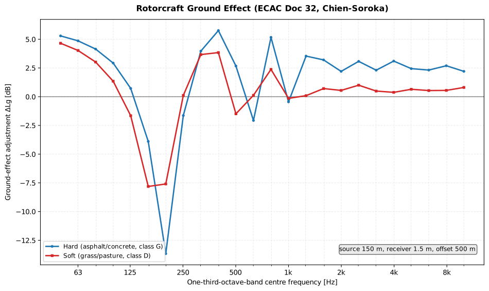
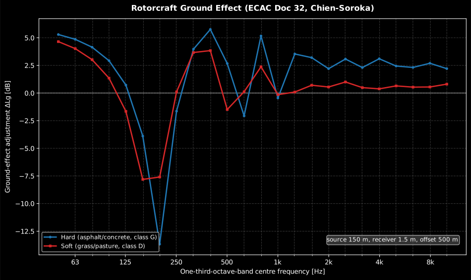
Show the code for this figure

import matplotlib.pyplot as plt
import numpy as np
from phonometry import aircraft

freqs = 1000.0 * 10.0 ** (np.arange(-13, 11) / 10.0)   # 50 Hz-10 kHz thirds
hs, hr, dp = 150.0, 1.5, 500.0                          # overflight geometry
grass = aircraft.ground_effect_adjustment(freqs, hs, hr, dp, flow_resistivity="D")
asphalt = aircraft.ground_effect_adjustment(freqs, hs, hr, dp, flow_resistivity="G")

fig, ax = plt.subplots()
ax.axhline(0.0, color="0.5", linewidth=1.0)
ax.semilogx(freqs, asphalt, marker="o", markersize=3,
            label="Hard (asphalt/concrete, class G)")
ax.semilogx(freqs, grass, marker="s", markersize=3,
            label="Soft (grass/pasture, class D)")
ax.set(xlabel="One-third-octave-band centre frequency [Hz]",
       ylabel="Ground-effect adjustment ΔLg [dB]",
       title="Rotorcraft ground effect (ECAC Doc 32, Chien-Soroka)")
ax.grid(True, which="both", alpha=0.3)
ax.legend()
plt.show()

import numpy as np
from phonometry import aircraft

freqs = 1000.0 * 10.0 ** (np.arange(-13, 11) / 10.0)   # 50 Hz-10 kHz thirds
r = 500.0
received = (lv
            + aircraft.spherical_spreading_adjustment(r)
            + aircraft.atmospheric_adjustment(freqs, r)
            + aircraft.ground_effect_adjustment(freqs, 150.0, 1.5, 500.0, flow_resistivity="D"))

The standard database is recorded at 60 m, the default. If a hemisphere uses a different polar distance (h.distance, e.g. 70 m hover rings), pass it to both distance-dependent adjustments as reference_distance=h.distance.

Flight conditions: interpolating between hemispheres

A database records one hemisphere per flight condition (airspeed V, path angle γ). Real conditions rarely coincide with a measured one, so the NORAH2 guidance interpolates (Eq. 3-10): both axes are normalised by their database spans (with the empirical factor Ffc = 2 on the path angle), a Delaunay triangulation covers the normalised conditions, and a query inside the convex hull blends its enveloping triangle with inverse-distance weights in the energy domain. Outside the hull the nearest condition is adopted unblended, which is also the behaviour ECAC Doc 32, 1st ed. prescribes for its whole envelope (it defines no interpolation yet).

from phonometry import aircraft

speeds = [50.0, 70.0, 60.0]                # one hemisphere per condition
angles = [0.0, 0.0, 10.0]                  # path angles, degrees
weights = aircraft.flight_condition_weights(speeds, angles, 60.0, 2.5)
lv = aircraft.interpolated_source_level(
    [h_50_level, h_70_level, h_60_climb], speeds, angles,
    60.0, 2.5, 0.0, 90.0)                  # blended level per band

The airspeed, not the ground speed, selects the hemisphere; the weights are unit-invariant as long as the query matches the database units. A database lookup triangulation can be passed as triangles (the NORAH database ships one per type; the shipped tables triangulate the raw (V, γ) plane, so passing them reproduces the reference implementation bin for bin). Mirrored-rotor class members substitute h.mirrored() (Eq. 2, φ → −φ) and certification-level offsets enter as level_offset.

Flight-path kinematics

flight_path_kinematics derives, from a time-stamped track by central finite differences, everything the event needs (Eq. 16-21 / Doc 32 Eq. 8-10): ground speed, airspeed (zero wind), heading, curvature, bank angle Φ = atan(K·Vg²/g) and path angle γ = atan(ΔZ/ΔS). The guidance recommends smoothing radar tracks (e.g. spline resampling to a 0.5 s cadence) before differentiating.

kin = aircraft.flight_path_kinematics(times, positions)   # positions (N, 3), m
kin.airspeed, kin.path_angle          # select the hemisphere per point
kin.bank_angle                        # tilts the hemisphere in turns
kin.plot()                            # speed and angle profiles

The single event: SEL, LASmax and EPNL

rotorcraft_event_level runs the whole chain for one flyover at one receiver: per track point the flight condition selects (or blends) the hemispheres, the emission angles address the source level (the frame is oriented by the heading and tilted by the bank angle in turns; pitch attitude is implicit in the hemispheres), and the received one-third-octave history is expressed at recorded time tr = te + r/c (Eq. 22, c = 346.1 m/s) and integrated: LASmax, SEL over the full history and over the certification 10 dB-down window (Doc 32 Eq. 27), and EPNL per ICAO Annex 16 (Doc 32 Eq. 28).

res = aircraft.rotorcraft_event_level(
    hemispheres, speeds, angles,      # the database
    times, positions,                 # the track (m, z up)
    receiver=(120.0, 0.0),            # ground position of the microphone
    flow_resistivity="D")             # grass site
res.la_max, res.sel, res.epnl         # LASmax, SEL, EPNL
res.plot()                            # the LA(t) time history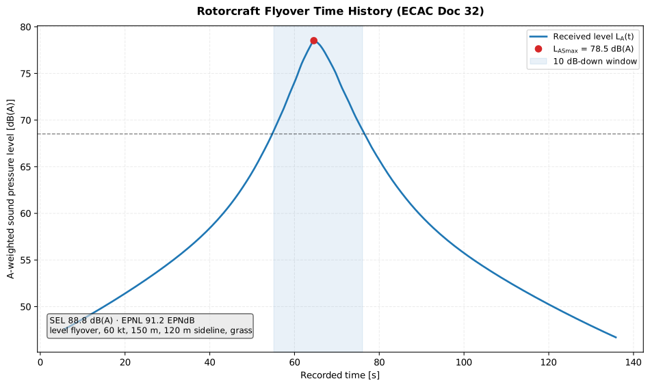

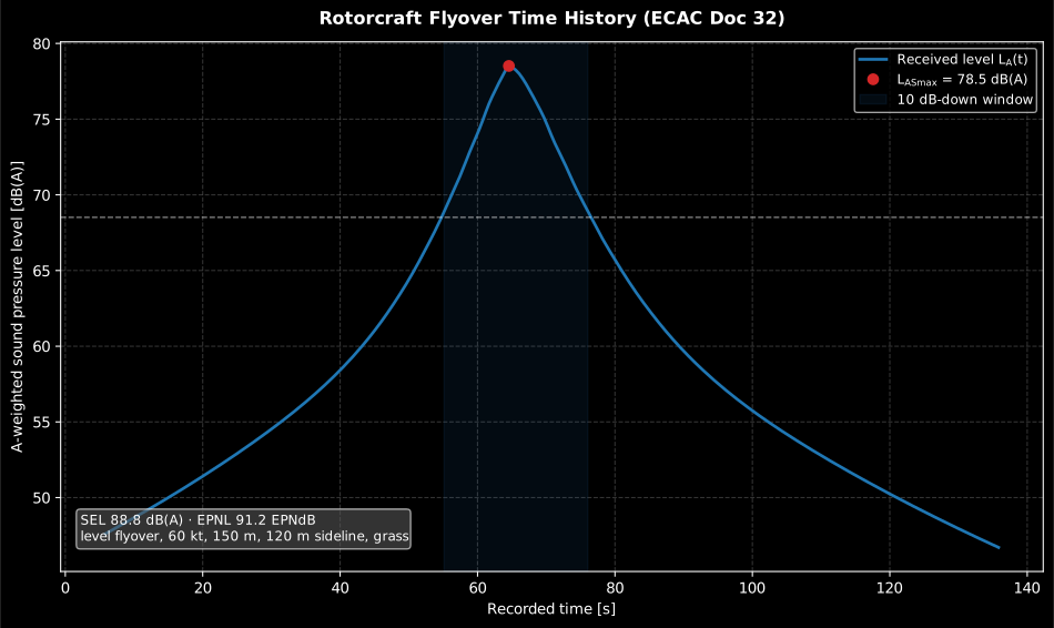
Show the code for this figure

import matplotlib.pyplot as plt
import numpy as np
from phonometry import aircraft

# A synthetic helicopter-like hemisphere on the standard 31-band, 10° grid.
freqs = 1000.0 * 10.0 ** (np.arange(-20, 11) / 10.0)   # 10 Hz-10 kHz thirds
az = np.arange(-90.0, 91.0, 10.0)
po = np.arange(0.0, 181.0, 10.0)
spectrum = 88.0 - 12.0 * np.log10(freqs / 100.0) ** 2   # broad low-mid hump
levels = (spectrum[None, None, :] - 0.045 * np.abs(po - 80.0)[None, :, None]
          - 0.02 * np.abs(az)[:, None, None])
h = aircraft.RotorcraftHemisphere(freqs, az, po, levels)

speed = 30.87                                           # 60 kt, in m/s
t = np.arange(0.0, 130.01, 0.5)
track = np.column_stack([np.zeros_like(t), speed * (t - 65.0),
                         np.full_like(t, 150.0)])
event = aircraft.rotorcraft_event_level(
    [h], [speed], [0.0], t, track, (120.0, 0.0), flow_resistivity="D")
event.plot()
plt.show()

Radar-track workflows can hand the smoothed per-point airspeed, path_angle, heading and bank_angle directly instead of deriving them from the positions; when they are derived, the track is in metres and seconds, so the database airspeeds must then be in m/s.

Ground-grid contours

rotorcraft_noise_contour evaluates the same event over a whole grid in one vectorised pass per emission step and reduces each receiver’s history to the SEL (metric="exposure") or LASmax (metric="maximum") footprint:

import numpy as np
from phonometry import aircraft

res = aircraft.rotorcraft_noise_contour(
    hemispheres, speeds, angles, times, positions,
    x=np.linspace(-2000.0, 2000.0, 81),
    y=np.linspace(-3000.0, 3000.0, 121),
    metric="exposure", flow_resistivity="D")
res.plot()                            # filled SEL contours

The ground may vary across the receivers without a full elevation model: flow_resistivity and ground_elevation accept one value per grid point (shape (len(y), len(x))), and each receiver’s two-ray model then uses its local values.

Terrain: the mean ground plane and screening

Doc 32, 1st ed., assumes flat terrain; its guidance adds the machinery for real sites. A varying vertical section is represented by its mean ground plane (Eq. 36-40), the least-squares line through the terrain polyline computed in closed form; source and receiver enter the flat-ground equations with their equivalent heights, measured orthogonally to that plane and floored at 0.1 m. Ground that changes type along the path averages its flow resistivity by the logarithm, weighted by segment length (Eq. 41).

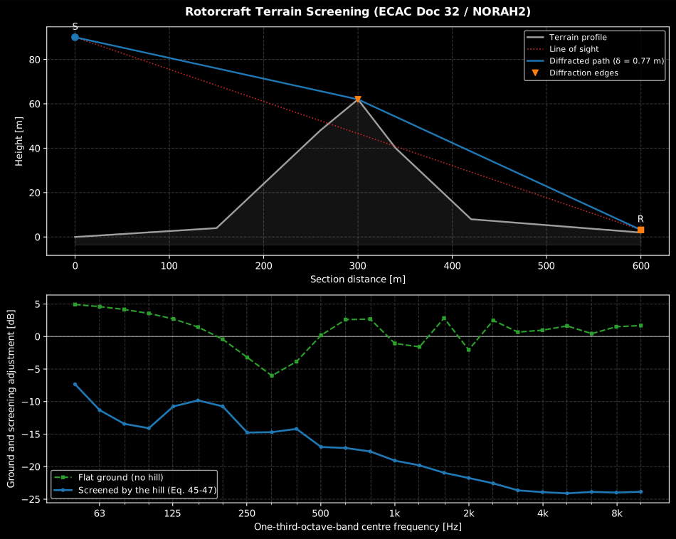
When terrain blocks the line of sight, the sound follows the shortest convex path over it (the guidance’s rubber band) and every touched vertex is a diffraction edge. The attenuation combines the pure diffraction of the path difference δ (Eq. 42-44, 10·Ch·log10(3 + (40/λ)·C″·δ), capped at 25 dB) with the source-side and receiver-side ground effects, each over its own mean ground plane and weighted by its image-path diffraction (Eq. 45-47, the CNOSSOS-EU scheme the guidance adopts). The ground effect is not evaluated separately in that regime.

mean_ground_plane, mean_flow_resistivity and diffraction_attenuation expose the pieces; terrain_screening_adjustment runs the whole section:

import numpy as np
from phonometry import aircraft

d = [0.0, 150.0, 260.0, 300.0, 340.0, 420.0, 600.0]     # section distances
z = [0.0, 4.0, 48.0, 62.0, 40.0, 8.0, 2.0]              # terrain heights
freqs = 1000.0 * 10.0 ** (np.arange(-13, 11) / 10.0)
res = aircraft.terrain_screening_adjustment(
    freqs, source=(0.0, 90.0), receiver=(600.0, 3.2), distances=d, heights=z,
    flow_resistivity="D")
res.screened, res.path_difference      # True, the rubber-band delta
res.adjustment                         # per band, replaces the flat-ground ΔLg
res.plot()                             # the section geometry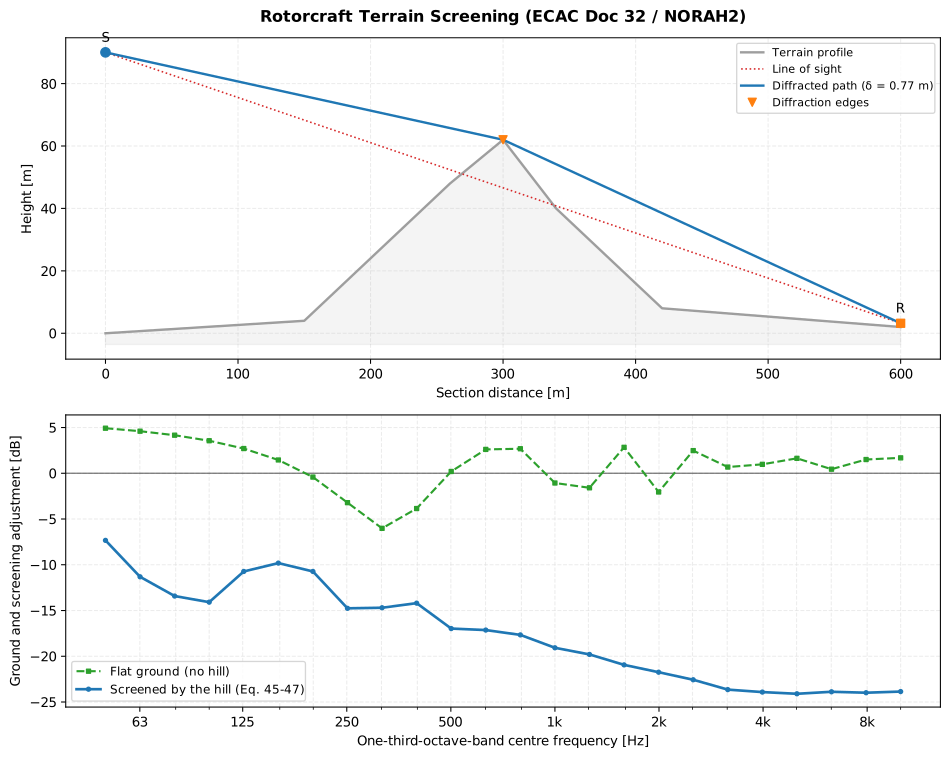

Show the code for this figure

import matplotlib.pyplot as plt
import numpy as np
from phonometry import aircraft

freqs = 1000.0 * 10.0 ** (np.arange(-13, 11) / 10.0)   # 50 Hz-10 kHz thirds
d = np.array([0.0, 150.0, 260.0, 300.0, 340.0, 420.0, 600.0])
z = np.array([0.0, 4.0, 48.0, 62.0, 40.0, 8.0, 2.0])
res = aircraft.terrain_screening_adjustment(
    freqs, (0.0, 90.0), (600.0, 3.2), d, z, flow_resistivity="D")
flat = aircraft.ground_effect_adjustment(freqs, 90.0, 1.2, 600.0,
                                         flow_resistivity="D")

fig, (ax, ax2) = plt.subplots(2, 1, figsize=(9, 7))
res.plot(ax=ax)
ax2.axhline(0.0, color="0.5", linewidth=1.0)
ax2.semilogx(freqs, flat, ls="--", marker="s", markersize=3,
             label="Flat ground (no hill)")
ax2.semilogx(freqs, res.adjustment, marker="o", markersize=3,
             label="Screened by the hill (Eq. 45-47)")
ax2.set(xlabel="One-third-octave-band centre frequency [Hz]",
        ylabel="Ground and screening adjustment [dB]")
ax2.grid(True, which="both", alpha=0.3)
ax2.legend()
plt.show()

The event and contour run over real sites by passing a digital elevation model: terrain=(x, y, z) on the track frame. Every emission-receiver pair then samples its own vertical section at terrain_resolution (default: the model’s cell size) and evaluates it with the machinery above; the receiver ground comes from the model. The cost grows with track points times grid points, so keep contour grids modest with terrain.

res = aircraft.rotorcraft_event_level(
    hemispheres, speeds, angles, times, positions, receiver=(1200.0, 300.0),
    terrain=(tx, ty, tz), flow_resistivity="D")

Validation

Validated against the NORAH2 guidance Table 4 (all 31 bands), the closed-form inverse-square spreading, the analytic rigid-ground and grazing limits of the ground effect, off-node bilinear lookups on the reference hemispheres of all eleven rotorcraft types, hand-checked interpolation simplices, closed-form kinematics and the Lorentzian SEL − LASmax flyover integral, and end to end against the NORAH2 prototype’s ARP verification cases: emission angles to 0.01°, retarded times to 0.02 s, every step level of the hard-ground events to 0.08 dB(A) out to 18 km, LASmax to 0.03 dB, SEL to 0.05 dB over hard ground (0.4 dB over soft ground), the 187-microphone contour grid to 0.7 dB worst-case, PNLTM to 0.1 dB and EPNL to about 1.3 dB (the prototype’s sub-noy-floor perceived-noisiness policy differs from the published Annex 16 law). One documented divergence remains: at far range over soft ground the prototype damps the coherent two-ray interference of guidance Eq. 30 towards the incoherent sum (up to 4.9 dB on individual low-level steps beyond 7 km); neither Doc 32 nor the guidance contains such a term, and this implementation follows the published equations.

The terrain machinery is anchored in closed form: the mean ground plane is exact on linear and symmetric profiles, a flat section reproduces the flat-ground model to machine precision and an inclined plane its analytic rotation, the log-mean resistivity recovers the geometric mean, the grazing diffraction gives the classical 10·log10(3), and a hand-checked hill fixes the rubber-band path difference. Per-receiver ground handling validates end to end against the prototype’s ARP Case 3 (187 microphones, each on its own ground elevation: every step level to 0.08 dB(A), SEL/LASmax to 0.05 dB, the contour grid to 0.15 dB) and the mixed-ground Case 2 grid reproduces in a single per-receiver-resistivity call. The prototype’s public release does not include a reconstructible screening case (the frame of its terrain model could not be pinned to the published outputs), so the diffraction chain itself rests on the closed-form anchors and its CNOSSOS-EU lineage.

What this guide covers

Covered. The ECAC Doc 32 hemisphere method and the EASA NORAH2 equation- level guidance (§A.3-A.5): the noise hemisphere and its bilinear lookup (RotorcraftHemisphere, hemisphere_source_level), the three propagation adjustments (spherical_spreading_adjustment, atmospheric_adjustment, ground_effect_adjustment, the Chien-Soroka model with Delany-Bazley impedance and the CNOSSOS flow-resistivity classes), the flight-condition interpolation (flight_condition_weights, interpolated_source_level), the flight-path kinematics (flight_path_kinematics), the single-event SEL, LASmax and EPNL (rotorcraft_event_level), ground-grid contours (rotorcraft_noise_contour) and the terrain mean-ground-plane and diffraction-screening chain (mean_ground_plane, mean_flow_resistivity, diffraction_attenuation, terrain_screening_adjustment). Validated against the NORAH2 guidance Table 4, closed-form geometric and grazing limits, and end to end against the NORAH2 prototype’s ARP verification cases.

Not covered. Hover, idle and taxi source handling (guidance §A.3.5) remains outside the implementation: the hemisphere source model assumes a flyover, not a stationary or ground-idling rotorcraft.

See also

• API reference: aircraft.rotorcraft_noise.

References

• Chien, C. F., & Soroka, W. W. (1975). Sound propagation along an impedance plane. Journal of Sound and Vibration, 43(1), 9-20. https://doi.org/10.1016/0022-460X(75)90200-XThe two-ray interference solution over an impedance plane behind the ground-effect adjustment.
• Delany, M. E., & Bazley, E. N. (1970). Acoustical properties of fibrous absorbent materials. Applied Acoustics, 3(2), 105-116. https://doi.org/10.1016/0003-682X(70)90031-9The one-parameter flow-resistivity impedance model the ground effect evaluates.
• European Civil Aviation Conference. (2026). Report on standard method of computing rotorcraft noise contours (ECAC.CEAC Doc 32, 1st ed.). The standard rotorcraft contour method whose hemisphere source model and propagation adjustments this page implements. The linked PDF is the free download; the document is catalogued on the ECAC documents page (https://www.ecac-ceac.org/documents/ecac-documents-and-international-agreements).
• Kephalopoulos, S., Paviotti, M., & Anfosso-Lédée, F. (2012). Common noise assessment methods in Europe (CNOSSOS-EU) (EUR 25379 EN). Publications Office of the European Union. https://doi.org/10.2788/31776The flow-resistivity ground classes 'A'-'H' accepted by ground_effect_adjustment.
• Olsen, H., Tuinstra, M., & van Oosten, N. (2024). Rotorcraft noise modelling guidance (Research Project NOISE SC01, deliverable D1.5d, contract EASA.2020.FC.06). European Union Aviation Safety Agency. The equation-level guidance (Eq. 13-35) behind the implementation, with the Table 4 attenuation values and the reference hemispheres used as oracles. Implemented scope (§A.3-A.5): the noise hemisphere, spherical spreading, atmospheric attenuation (ISO 9613-1, Table 4), the Chien-Soroka ground effect (Delany-Bazley impedance, CNOSSOS flow resistivity), the flight-condition interpolation (Eq. 3-10), the flight-path kinematics (Eq. 16-21 / Doc 32 Eq. 8-10), recorded time (Eq. 22), the single-event metrics SEL/LASmax and EPNL (Doc 32 Eq. 27/28, ICAO Annex 16 App. 2), the mean ground plane and equivalent heights (Eq. 36-40), the log-mean flow resistivity (Eq. 41) and the terrain screening chain (Eq. 42-47 with the guidance's noise-path appendices; CNOSSOS-EU lineage). Hover, idle and taxi source handling (§A.3.5) remains outside the implementation. The linked PDF is the free download; the project is catalogued on the EASA project page (https://www.easa.europa.eu/en/research-projects/environmental-research-rotorcraft-noise).