Programme loudness and true peak (BS.1770 / EBU R 128)

ITU-R BS.1770-5 defines how broadcast and streaming measure the loudness of a programme: K-weighting, mean-square power in gated 400 ms blocks and a channel-weighted sum, reported in LKFS/LUFS. EBU R 128 builds the normalisation practice on top of it (every programme is levelled to −23.0 LUFS with a true-peak ceiling of −1 dBTP), and its companions EBU Tech 3341 and Tech 3342 add the EBU Mode meter (momentary, short-term and integrated loudness) and the loudness range (LRA). phonometry implements the full chain in the broadcast namespace and validates every synthesizable EBU test signal against its official tolerance.

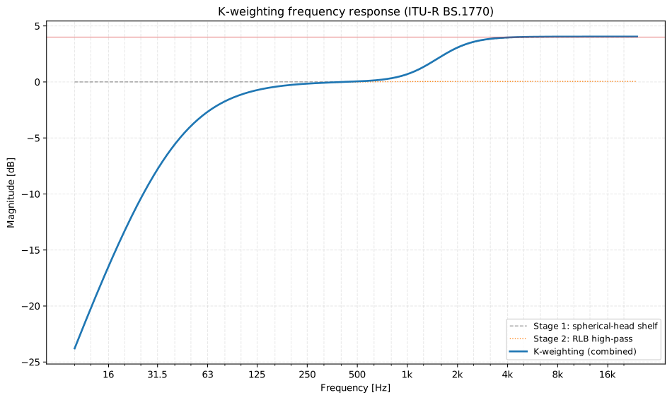
1. K-weighting and the loudness measure (Annex 1)

The signal first passes a two-stage pre-filter: a ~+4 dB high-frequency shelf modelling the head as a rigid sphere, then the RLB high-pass. The concatenation is the K-weighting. The loudness over an interval is the channel-weighted sum of the mean-square powers $z_i$ (Formula 2):

$$L_K=-0.691+10{\log }_{10}\sum _i{G}_i{z}_i\text{LKFS},$$

where the constant cancels the K-weighting gain at 997 Hz and $G_i$ weighs each channel (1.0 for the front channels, 1.41 for the surrounds, LFE excluded, Table 3). The Recommendation anchors the scale: a 0 dB FS 997 Hz sine on one front channel reads −3.01 LKFS. The unit is written LKFS by the ITU and LUFS by the EBU; they are identical, and 1 LU is 1 dB.

import numpy as np
from phonometry import broadcast

fs = 48000
t = np.arange(20 * fs) / fs
x = np.zeros((5, t.size))                     # L, R, C, Ls, Rs
x[0] = np.sin(2 * np.pi * 997.0 * t)          # 0 dB FS on the left channel
print(round(broadcast.integrated_loudness(x, fs), 2))   # -3.01  LKFS

The biquad coefficients are tabulated at 48 kHz (Tables 1-2) and returned verbatim at that rate; any other rate re-derives them through the analog prototype so the response matches the specification (within 0.02 dB at 32 kHz and above; rates below 16 kHz are rejected):

import numpy as np
from phonometry import broadcast

(b1, a1), (b2, a2) = broadcast.k_weighting_coefficients(48000)
print(b1)   # [ 1.53512486 -2.69169619  1.19839281]  (Table 1, verbatim)
y = broadcast.k_weighting(np.random.default_rng(0).standard_normal(48000),
                          48000)              # the filtered signal itself

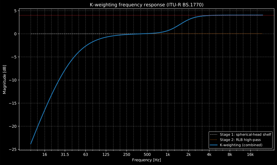
k_weighting_response evaluates those same biquads as a transfer function and returns a frozen KWeightingResponse carrying the combined magnitude (magnitude_db) and the two stages (shelf_db, highpass_db) over a logarithmic frequency grid; its .plot() draws the response, with the +4 dB spherical-head shelf and the RLB high-pass roll-off:

Show the code for this figure

import matplotlib.pyplot as plt
from phonometry import broadcast

broadcast.k_weighting_response(48000).plot()
plt.show()

2. Gating and the programme loudness

The integrated (programme) loudness divides the measurement into gating blocks of 400 ms overlapping 75 % and gates them twice (Formulae 3-7): blocks below the absolute threshold −70 LKFS are dropped; the loudness of the survivors minus 10 LU sets the relative threshold, and the blocks above both gates define the result. The gate keeps long quiet passages (atmosphere, pauses, applause tails) from dragging the level of the foreground down:

import numpy as np
from phonometry import broadcast

fs = 48000
def tone(level_dbfs, seconds):
    t = np.arange(int(seconds * fs)) / fs
    return 10 ** (level_dbfs / 20) * np.sin(2 * np.pi * 1000.0 * t)

# 10 s of programme at -23 dBFS followed by 30 s of quiet ambience.
x = np.concatenate([tone(-23.0, 10.0), tone(-50.0, 30.0)])
res = broadcast.program_loudness(np.vstack([x, x]), fs)
print(round(res.integrated, 1))            # -23.1  LUFS (the tail is gated)
print(round(res.relative_threshold, 1))    # -39.0  LUFS
res.plot()   # the loudness trace: the integrated line ignores the tail (needs matplotlib)

An ungated mean over the same 40 s would sit near −29 LUFS: the gating is what makes wide-loudness-range programmes match on air. EBU R 128 normalises this integrated value to −23.0 LUFS; where the target is not practically achievable (live programmes, for example) a tolerance of ±1.0 LU is permitted, and quality-control workflows allow ±0.2 LU for measurement error. The figure makes the gate visible on a shaped-noise programme with a long quiet tail:

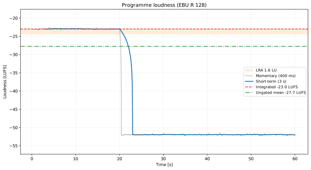
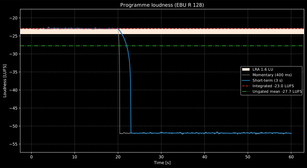
The relative gate (10 LU below the survivors) drops every block of the tail, so the integrated loudness holds the foreground at −23.0 LUFS while the ungated energy mean sinks towards −27.7 LUFS — and would keep sinking with every extra minute of ambience. Without the gate, quiet passages would let the foreground of a film mix ride far above the target.

Show the code for this figure

import matplotlib.pyplot as plt
import numpy as np
from scipy import signal
from phonometry import broadcast

fs = 48000
rng = np.random.default_rng(3341)
sos = signal.butter(2, 2000.0, fs=fs, output="sos")
chunks = []
# 20 s of programme material, then 40 s of quiet room ambience ~29 LU lower.
for level, seconds in [(-23.0, 20.0), (-52.0, 40.0)]:
    noise = signal.sosfilt(sos, rng.standard_normal(int(seconds * fs)))
    noise /= np.sqrt(np.mean(noise ** 2))
    chunks.append(10 ** (level / 20) * noise)
x = np.concatenate(chunks)
# Loudness-normalise the programme to the R 128 target, then meter it.
x *= 10 ** ((-23.0 - broadcast.integrated_loudness(np.vstack([x, x]), fs)) / 20)
res = broadcast.program_loudness(np.vstack([x, x]), fs)

ax = res.plot()
finite = res.momentary[np.isfinite(res.momentary)]
ungated = 10 * np.log10(np.mean(10 ** (finite / 10)))
ax.axhline(ungated, ls="-.", color="#2ca02c",
           label=f"Ungated mean {ungated:.1f} LUFS")
ax.legend(loc="center right")
plt.show()

3. EBU Mode: momentary, short-term, integrated

EBU Tech 3341 defines the three time scales of a compliant meter, and one call computes them all:

• Momentary (M): sliding 400 ms window, no gating;
• Short-term (S): sliding 3 s window, no gating;
• Integrated (I): the gated programme loudness above,

plus Max M and Max S, the true peak and the LRA:

import numpy as np
from phonometry import broadcast

fs = 48000
def tone(level_dbfs, seconds):
    t = np.arange(int(seconds * fs)) / fs
    return 10 ** (level_dbfs / 20) * np.sin(2 * np.pi * 1000.0 * t)

# EBU Tech 3341 test case 3: -36 / -23 / -36 dBFS steps.
x = np.concatenate([tone(-36.0, 10.0), tone(-23.0, 60.0), tone(-36.0, 10.0)])
res = broadcast.program_loudness(np.vstack([x, x]), fs)
print(round(res.integrated, 1), round(res.max_momentary, 1),
      round(res.max_short_term, 1))         # -23.0 -23.0 -23.0
res.plot()   # M/S traces, integrated line and LRA band (needs matplotlib)

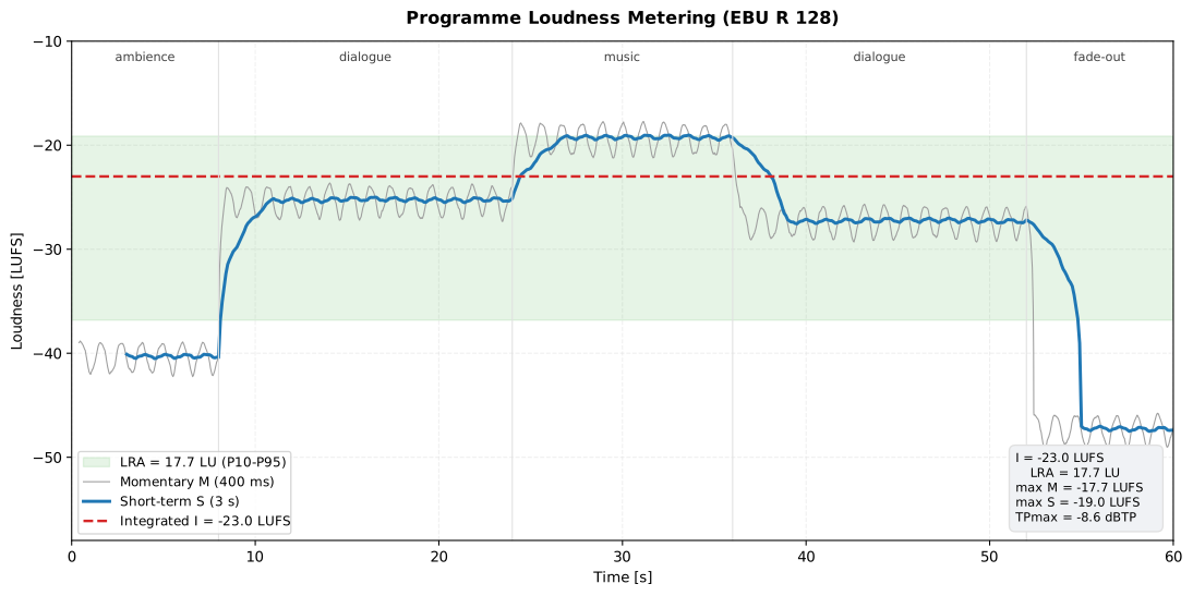
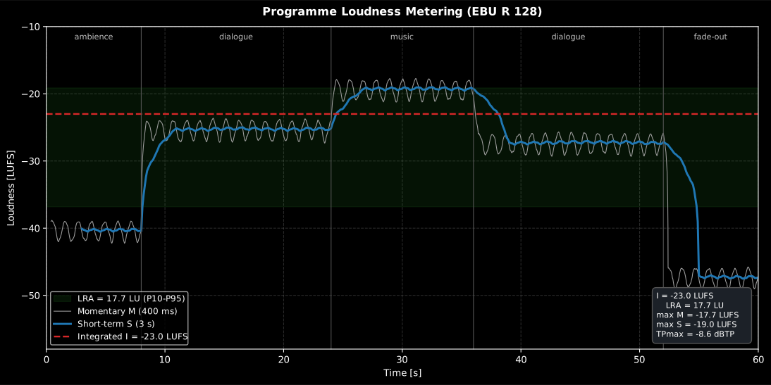
The frozen ProgramLoudnessResult carries the M and S series with their time axes, the maxima, the thresholds, the LRA with its percentile edges, the per-channel true peaks and the channel weights; its .plot() draws the loudness trace of the programme:

Show the code for this figure

import matplotlib.pyplot as plt
import numpy as np
from scipy import signal
from phonometry import broadcast

fs = 48000
rng = np.random.default_rng(1770)
sos = signal.butter(2, 2000.0, fs=fs, output="sos")
chunks = []
for level, seconds in [(-38, 8), (-23, 16), (-17, 12), (-25, 16), (-45, 8)]:
    noise = signal.sosfilt(sos, rng.standard_normal(int(seconds * fs)))
    noise /= np.sqrt(np.mean(noise ** 2))
    t = np.arange(noise.size) / fs
    wobble = 1 + 0.22 * np.sin(2 * np.pi * 0.9 * t) \
        + 0.14 * np.sin(2 * np.pi * 2.83 * t + 1.0)
    chunks.append(10 ** (level / 20) * noise * wobble)
x = np.concatenate(chunks)

# Normalise the programme to the R 128 target, then meter it.
gain = -23.0 - broadcast.integrated_loudness(np.vstack([x, x]), fs)
x *= 10 ** (gain / 20)
broadcast.program_loudness(np.vstack([x, x]), fs).plot()
plt.show()

4. Loudness range (EBU Tech 3342)

The loudness range quantifies how much the loudness varies on a macroscopic time scale, in LU. It is the spread between the 10th and 95th percentiles of the short-term loudness distribution after a cascaded gate: an absolute threshold at −70 LUFS, then a relative threshold −20 LU below the level of what survived (deliberately deeper than the −10 LU of the integrated measure, so quiet-but-real foreground still counts). The percentiles keep a single gunshot or a fade-out from inflating the value:

import numpy as np
from phonometry import broadcast

fs = 48000
def tone(level_dbfs, seconds):
    t = np.arange(int(seconds * fs)) / fs
    return 10 ** (level_dbfs / 20) * np.sin(2 * np.pi * 1000.0 * t)

# EBU Tech 3342 test case 1: 20 s at -20 dBFS, then 20 s at -30 dBFS.
x = np.concatenate([tone(-20.0, 20.0), tone(-30.0, 20.0)])
res = broadcast.program_loudness(np.vstack([x, x]), fs)
print(round(res.loudness_range, 1))         # 10.0  LU
res.plot()   # the shaded LRA band spans the P10-P95 spread (needs matplotlib)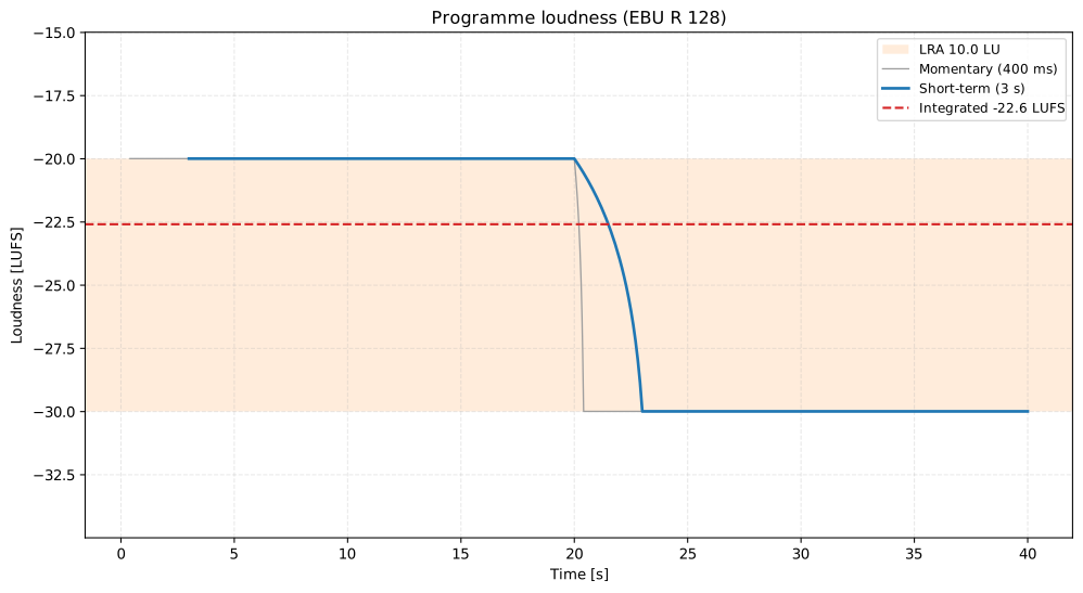

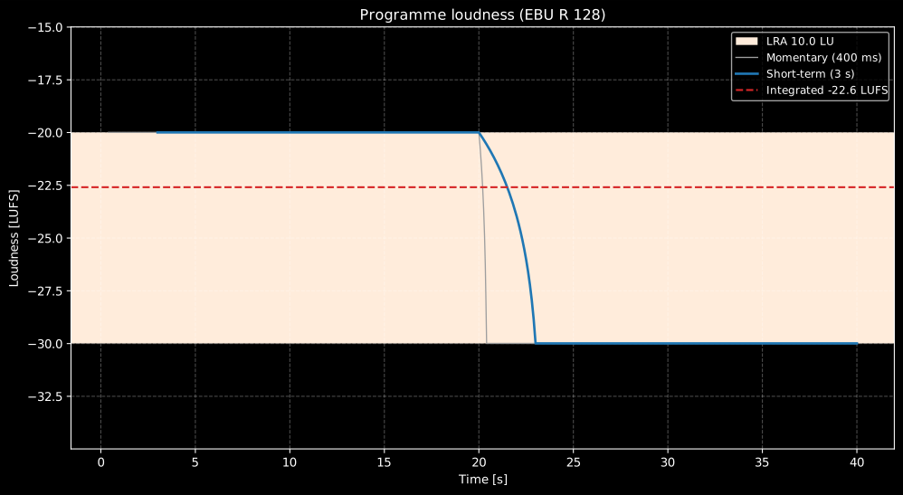
On the Tech 3342 reference case the short-term distribution has two plateaus 10 LU apart, and the shaded band between the 10th and 95th percentile edges reads exactly LRA = 10.0 LU; the integrated loudness settles between the plateaus. On real programmes the same band tells a dialogue-normalised drama (LRA around 10-20 LU) from a compressed commercial (a few LU) at a glance.

Show the code for this figure

import matplotlib.pyplot as plt
import numpy as np
from phonometry import broadcast

fs = 48000
def tone(level_dbfs, seconds):
    t = np.arange(int(seconds * fs)) / fs
    return 10 ** (level_dbfs / 20) * np.sin(2 * np.pi * 1000.0 * t)

# EBU Tech 3342 test case 1: 20 s at -20 dBFS, then 20 s at -30 dBFS.
x = np.concatenate([tone(-20.0, 20.0), tone(-30.0, 20.0)])
res = broadcast.program_loudness(np.vstack([x, x]), fs)
res.plot()   # the LRA band spans exactly the 10 LU between the plateaus
plt.show()

loudness_range() is also available standalone on any short-term loudness vector, following the Tech 3342 reference implementation (including its nearest-rank percentile indexing). The EBU does not recommend LRA for programmes shorter than a minute: too few 3 s windows.

5. True peak (Annex 2)

Digital sample peaks lie: the true maximum of the reconstructed waveform generally falls between samples, and a sample-peak meter under-reads a badly phased tone at $f_s/4$ by 3 dB (worst case $20{\log }_{10}\cos (\pi f_{\mathrm{norm}}/n)$ for oversampling ratio $n$). BS.1770-5 Annex 2 therefore meters the true peak on a signal oversampled to at least 192 kHz (4× at 48 kHz), in dBTP (dB relative to 100 % full scale):

import numpy as np
from phonometry import broadcast

fs = 48000
t = np.arange(fs) / fs
# A full-scale fs/4 tone whose peaks fall exactly between samples.
x = np.sin(2 * np.pi * (fs / 4) * t + np.pi / 4)
print(round(float(broadcast.true_peak_level(x, fs, oversample=1)), 2))  # -3.01
print(round(float(broadcast.true_peak_level(x, fs)), 2))                #  0.12

The interpolator recovers the inter-sample excursion the sample grid missed (the residual +0.12 dB is interpolation ripple from the abrupt tone edges, inside the +0.2/−0.4 dB tolerance that EBU Mode meters must meet). EBU R 128 caps production at −1 dBTP; distribution codecs often need more headroom. This is the same oversampled-peak machinery behind the C-weighted lc_peak of Integrated & Statistical Levels.

6. Multichannel programmes and Annex 3

With 1, 2, 5 or 6 channels the Table 3 weights apply automatically (channel order L, R, C, Ls, Rs, or L, R, C, LFE, Ls, Rs with the LFE excluded). For any other loudspeaker layout (22.2, 4+7+0 and the rest of the BS.2051 advanced sound systems), Annex 3 derives the weight of each channel from its loudspeaker position: 1.41 (+1.5 dB) for mid-layer side loudspeakers (60° ≤ |azimuth| ≤ 120°, |elevation| < 30°), 1.0 elsewhere:

from phonometry import broadcast

print(broadcast.channel_weight(110.0, 0.0))    # 1.41  (M+110, side)
print(broadcast.channel_weight(110.0, 35.0))   # 1.0   (U+110, upper layer)
weights = broadcast.channel_weight([0, 30, -30, 90, -90], [0, 0, 0, 0, 0])
# -> [1. 1. 1. 1.41 1.41]; pass as program_loudness(..., weights=weights)

Object-based audio (Annex 4) is measured by rendering to a loudspeaker configuration first and metering the render; the rendering itself is out of scope here.

EBU R 128 report (.report())

ProgramLoudnessResult.report(path) renders a one-page PDF compliance fiche laid out like a broadcast loudness-delivery sheet: a standard-basis line, an optional metadata header block, a full-width compliance table (Metric | Measured | Target / Limit | Result) and, below it, the full-width loudness-vs-time plot (the result’s own .plot(), with the momentary and short-term traces, the integrated line and the LRA band). The verdict is driven only by the integrated loudness and the maximum true peak; the loudness range and the momentary/short-term maxima are shown as informational rows (an en dash in the Result column, never a pass/fail colour). A boxed I = X LUFS (LRA = Y LU, max TP = Z dBTP) single number, a combined PASS/FAIL verdict and a footer with the fixed disclaimer close the sheet.

The stacked layout (compliance table on top, plot below) differs from the narrow two-panel body of the other fiches because the compliance table needs four columns and the loudness-vs-time trace is landscape. It uses the same ReportMetadata container and rendering engine as the ISO 717 insulation fiche; a supplied requirement is read as the target programme loudness in LUFS (defaulting to the EBU R 128 −23.0 LUFS), and the fiche passes when the integrated loudness is within the selected R 128 tolerance of it and the true peak is at or below −1.0 dBTP. The tolerance follows the tolerance keyword: the default "qc" applies the ±0.2 LU measurement-error allowance of R 128 item i) (loudness workflows such as Quality Control), and "live" applies the ±1.0 LU tolerance of item h), permitted only where the Target Level is not achievable practically (live programmes, for example); the applied rule and its R 128 item are printed on the fiche. The verdict is evaluated on the loudness rounded to the displayed 0.1 LU, so the printed numbers can never contradict it. Rendering needs reportlab (pip install phonometry[report]); only engine="reportlab" is supported. The fiche renders in English by default; pass language="es" for a Spanish fiche (translated fixed strings and a comma decimal separator), e.g. res.report("loudness_fiche_es.pdf", language="es").

from phonometry import broadcast, ReportMetadata

res = broadcast.program_loudness(x, fs)   # a finished stereo programme
res.report(
    "loudness_fiche.pdf",
    metadata=ReportMetadata(
        specimen="Reference tone sequence",
        measurement_standard="EBU R 128",
        laboratory="Phonometry Reference Laboratory",
        requirement=-23.0,                # target programme loudness (LUFS)
    ),
)                                          # I (LUFS), LRA (LU), true peak (dBTP)

The example fiche is regenerated with make reports and kept rendered in the repository; click the preview to open the PDF.

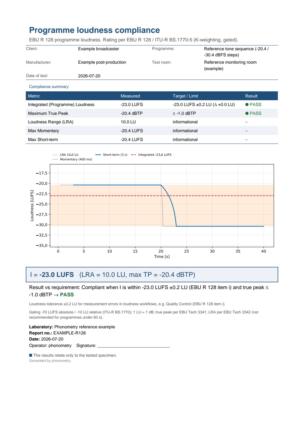
One-page programme-loudness compliance fiche: a metadata header, a four-column compliance table with the integrated loudness and maximum true peak carrying the verdict and the loudness range and momentary/short-term maxima as informational rows, the full-width loudness-vs-time plot, the boxed I = -23.0 LUFS (LRA = 10.0 LU, max TP = -20.4 dBTP) single-number result and a PASS verdict against the -23.0 LUFS target under the default ±0.2 LU QC tolerance of EBU R 128 item i).

Download the report (PDF)

Programme-loudness compliance fiche (ProgramLoudnessResult.report), I in LUFS with LRA in LU and true peak in dBTP.

7. Validation

Every synthesizable “minimum requirements” signal of EBU Tech 3341 (cases 1-6 and 9-23) and Tech 3342 (cases 1-4) runs in the test suite with its official tolerance (±0.1 LU for loudness, +0.2/−0.4 dB for true peak, ±1 LU for LRA), alongside the 997 Hz anchor and the closed-form under-read bound of Annex 2 Attachment 1. Cases 7-8 and the LRA cases 5-6 use authentic programme material distributed by the EBU and are not synthesizable; they run against the official EBU loudness test set (fetched from the EBU, whose licence covers technical testing only, so the audio is never committed) and all four pass within tolerance; the per-block loudness series measured from them are committed as plain data, so the gating and LRA stages of these cases also run everywhere without the audio. The independent pyloudnorm meter is a useful cross-check for real recordings; it was not used as a source for this implementation.

What this guide covers

Covered. ITU-R BS.1770-5 Annex 1: the K-weighting pre-filter of Tables 1-2, and the channel-weighted integrated loudness with its two-stage gate (Formulae 1-7, Table 3). k_weighting, k_weighting_coefficients and program_loudness implement these. Annex 2’s oversampled true-peak level runs through true_peak_level. Annex 3’s position-dependent channel weights for advanced sound systems run through channel_weight. EBU R 128’s −23.0 LUFS target and −1 dBTP ceiling sit on top of that. EBU Tech 3341’s momentary/short-term/integrated meter and EBU Tech 3342’s loudness range come from the same program_loudness result, with loudness_range() also standalone.

Not covered. BS.1770-5 Annex 4, object-based audio, is out of scope. The guide notes that rendering to a loudspeaker layout has to happen first, and phonometry implements no spatial-audio renderer for that step. EBU Tech 3343 is cited only as production practice around these numbers: guidance, not an algorithm, and nothing here runs it.

References

• European Broadcasting Union. (2023). Guidelines for production of programmes in accordance with EBU R 128 (EBU Tech 3343). The production practice around the numbers on this page.
• European Broadcasting Union. (2023). Loudness metering: 'EBU Mode' metering to supplement loudness normalisation (EBU Tech 3341). The EBU Mode momentary/short-term/integrated (M/S/I) time scales, validated against the synthesizable Table 1 minimum-requirements test signals with their official tolerances.
• European Broadcasting Union. (2023). Loudness normalisation and permitted maximum level of audio signals (EBU R 128). The −23.0 LUFS target level, the −1 dBTP ceiling and the normalisation practice.
• European Broadcasting Union. (2023). Loudness range: A measure to supplement loudness normalisation (EBU Tech 3342). The loudness range (LRA) algorithm, its reference implementation and its test signals, validated against its Table 1 signals at ±1 LU.
• International Telecommunication Union. (2023). Algorithms to measure audio programme loudness and true-peak audio level (Recommendation ITU-R BS.1770-5 (11/2023)). The K-weighting pre-filter (Annex 1, Tables 1-2), the channel-weighted loudness and two-stage gating (Annex 1, Formulae 1-7, Table 3), the true-peak estimation guidelines (Annex 2 and its Attachment 1 under-read bound) and the position-dependent channel weights for advanced sound systems (Annex 3, Tables 4-5).
• Steinmetz, C. J., & Reiss, J. D. (2021). pyloudnorm: A simple yet flexible loudness meter in Python. 150th AES Convention. An independent BS.1770 implementation, useful as a cross-check.