Impulsive-sound prominence (NT ACOU 112)
Standards: NT ACOU 112ISO 1996ISO/PAS 1996
Noise with prominent impulses (hammering, riveting, pile driving) is more
annoying than a steady sound of the same equivalent level. NT ACOU 112:2002
(a Nordtest method) quantifies how prominent an impulse is and turns it into a
graduated adjustment KI added to the measured LAeq. The prominence is read
from two properties of each impulse’s onset in the A-weighted, time-weighting-F
level history: how fast it rises (the onset rate) and how far it rises (the
level difference).
1. Predicted prominence (clause 7)
Section titled “1. Predicted prominence (clause 7)”For each candidate impulse the predicted prominence P combines the onset
rate (in dB/s) and the level difference (in dB) on a logarithmic scale
(Formula 1):
The coefficients were fitted to listening tests and P is designed to peak
around 15 for very sudden, loud impulses. The impulse with the highest P
over a 30-minute period governs. A level rise only qualifies as an impulse
when its onset rate exceeds 10 dB/s (clause 4.5; clause 8 applies the
adjustment “for sounds with onset rates larger than 10 dB/s” only):
impulse_prominence marks non-qualifying events in its qualifies mask,
warns about them, and never lets them set the governing prominence or a
KI (the adjustment is 0 dB when no event qualifies).
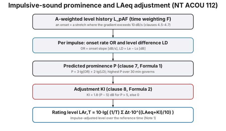
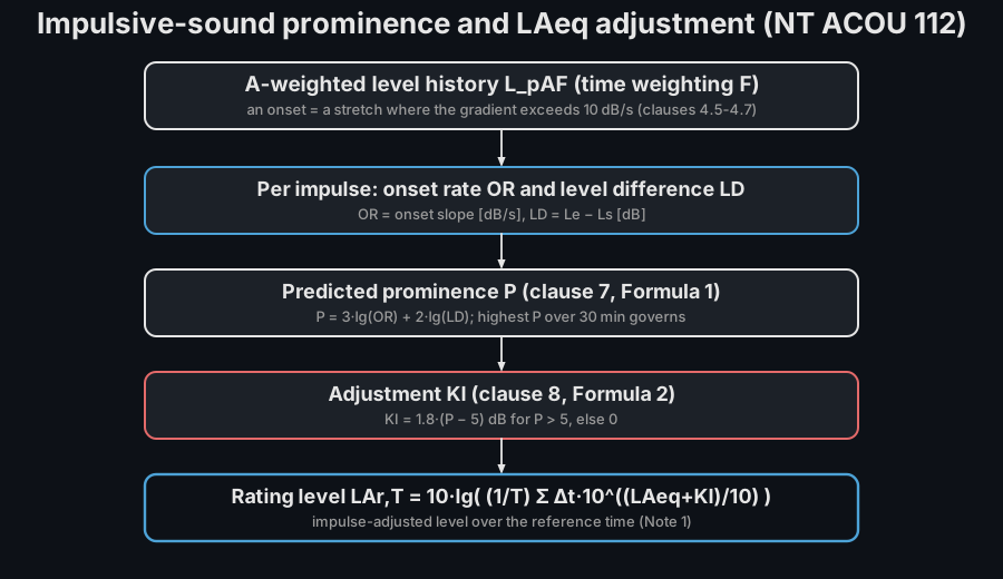
A magnifier scans the A-weighted Fast level history L_AF; where the level climbs faster than 10 dB/s the onset stretch is highlighted, and the onset rate (200 dB/s), level difference (30 dB), prominence P and adjustment KI boxes light up in turn.
A magnifier scans the A-weighted Fast level history L_AF; where the level climbs faster than 10 dB/s the onset stretch is highlighted, and the onset rate (200 dB/s), level difference (30 dB), prominence P and adjustment KI boxes light up in turn.
from phonometry import environmental
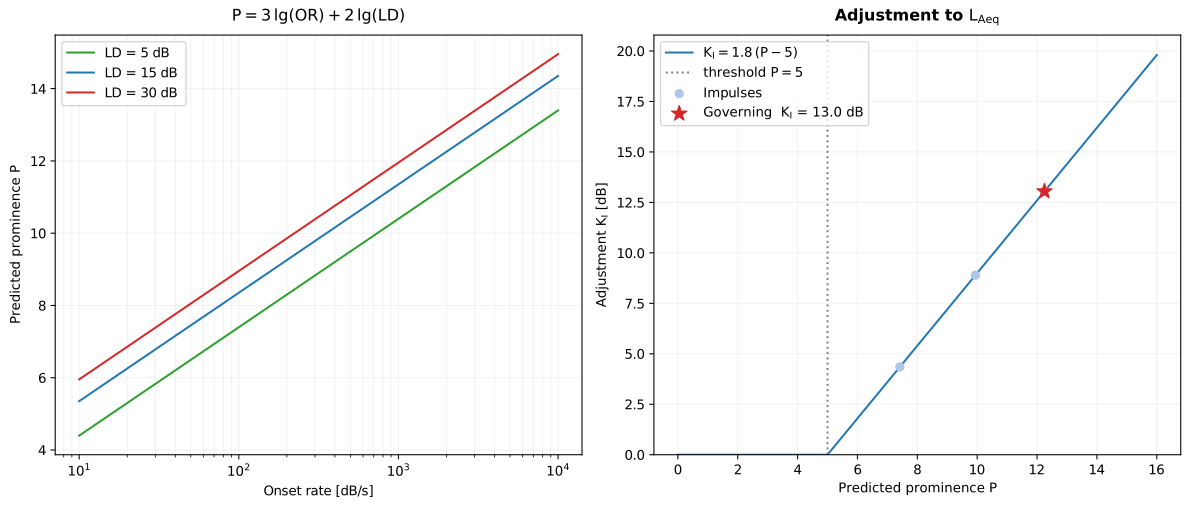
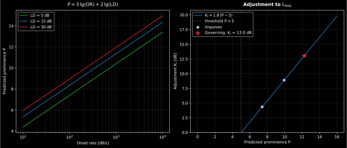
# Three candidate impulses: (onset rate dB/s, level difference dB).result = environmental.impulse_prominence([1200.0, 300.0, 60.0], [32.0, 18.0, 11.0])print(result.per_impulse.round(2))  # [12.25  9.94  7.42]print(round(result.prominence, 2))  # 12.25  (the governing impulse)print(round(result.adjustment, 2))  # 13.05  dB
result.plot()   # the KI(P) curve of section 2 with these impulses marked
A single impulse can be evaluated directly with predicted_prominence:
from phonometry import environmental
# P = 3*lg(1000) + 2*lg(30) = 9 + 2.95 = 11.95.print(round(environmental.predicted_prominence(1000.0, 30.0), 4))  # 11.9542
2. Adjustment to LAeq (clause 8)
Section titled “2. Adjustment to LAeq (clause 8)”Below a prominence of 5 the impulse is not audible enough to matter; above it the adjustment grows linearly (Formula 2):
from phonometry import environmental
print(float(environmental.impulse_adjustment(10.0)))  # 9.0 dBprint(float(environmental.impulse_adjustment(5.0)))   # 0.0 dB (at the threshold)
The adjustment is applied to LAeq,30min from the single event with the
highest prominence. The rating level over a longer reference time combines
the impulse-adjusted equivalent levels of the sub-intervals (clause 8, Note 1):
from phonometry import environmental
# Two 30-min periods: one impulsive (KI = 7.6 dB), one quiet.print(round(environmental.rating_level([72.0, 66.0], [7.6, 0.0], [30.0, 30.0], 60.0), 2))# 76.78 dB
The ImpulseProminenceResult carries the per_impulse prominences, the governing
prominence and its adjustment, and its .plot() draws the KI(P) curve
with the impulses marked. The method is a supplement to the environmental-noise
measurement of ISO 1996-2.
Show the code for this figure
import numpy as npimport matplotlib.pyplot as pltfrom phonometry import environmental
# One line for the adjustment curve with the impulses marked:environmental.impulse_prominence([1200.0, 300.0, 60.0], [32.0, 18.0, 11.0]).plot()plt.show()
# By hand, the left panel — P vs onset rate for three level differences:orate = np.logspace(1, 4, 200)for ld in (5.0, 15.0, 30.0):    plt.plot(orate, environmental.predicted_prominence(orate, np.full_like(orate, ld)),             label=f"LD = {ld:g} dB")plt.xscale("log"); plt.legend(); plt.show()
3. Objective measurement from a signal (ISO/PAS 1996-3)
Section titled “3. Objective measurement from a signal (ISO/PAS 1996-3)”NT ACOU 112 takes the onset rate and level difference as inputs. ISO/PAS
1996-3:2022 keeps the same prominence and adjustment formulae but adds the
objective measurement chain that reads those quantities straight from a
calibrated recording. impulsive_sound_adjustment A-weights the signal,
applies time weighting F ( = 125 ms), samples the level history LpAF
every 10-25 ms, detects each onset (the contiguous stretch whose gradient
exceeds 10 dB/s, merging events less than 50 ms apart), measures its level
difference LD = Le − Ls and its least-squares onset rate OR, and returns
the governing adjustment KI with the source category of clause 7:
not impulsive (KI = 0), regular impulsive (0 < KI ≤ 5) or
highly impulsive (KI > 5).
The onset detection can be exercised on a level history directly with
detect_onsets, which is convenient for meters that already log LpAF:
import numpy as npfrom phonometry import environmental
# An LpAF history sampled every 20 ms: quiet, a 30 dB rise over 0.30 s, steady.dt = 0.02levels = np.concatenate([    np.full(10, 40.0),    40.0 + 30.0 * np.arange(1, 16) / 15,   # a straight 100 dB/s onset to 70 dB    np.full(15, 70.0),])onset = environmental.detect_onsets(levels, dt)[0]print(round(onset.onset_rate), round(onset.level_difference))  # 100 30print(round(onset.prominence, 2))                              # 8.95
From a calibrated time signal (in pascal) the whole chain runs end to end:
result = environmental.impulsive_sound_adjustment(signal, fs)print(result.category)                  # e.g. 'highly impulsive'print(round(result.adjustment, 1))      # KI in dB (0.0 to about 9 dB in typical cases)print(round(result.adjusted_laeq, 1))   # LAeq + KI
result.plot()   # the LpAF history with the detected onsets (needs matplotlib)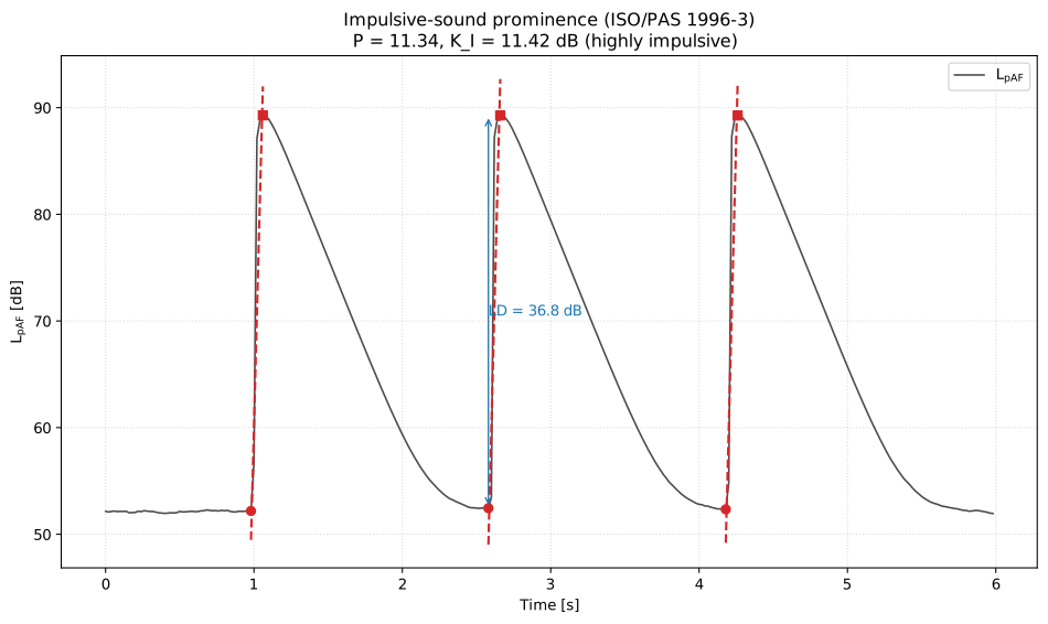
Show the code for this figure
import numpy as npimport matplotlib.pyplot as pltfrom phonometry import environmental
# Three hammer strikes over a 55 dB(A) background, 6 s at 48 kHz.fs = 48000rng = np.random.default_rng(7)t = np.arange(int(6.0 * fs)) / fsbackground = rng.standard_normal(t.size)background *= 2e-5 * 10 ** (55 / 20) / np.sqrt(np.mean(background ** 2))signal = background.copy()for onset_time in (1.0, 2.6, 4.2):    decay = np.exp(-(t - onset_time) / 0.08) * (t >= onset_time)    strike = decay * rng.standard_normal(t.size)    window = (t >= onset_time) & (t < onset_time + 0.1)    strike *= 2e-5 * 10 ** (95 / 20) / np.sqrt(np.mean(strike[window] ** 2))    signal += strike
res = environmental.impulsive_sound_adjustment(signal, fs)print(res.category, round(res.prominence, 2), round(res.adjustment, 2))# highly impulsive 11.34 11.42
# One line: the level history with the onsets, the fitted onset lines and# the governing level difference.res.plot()plt.show()
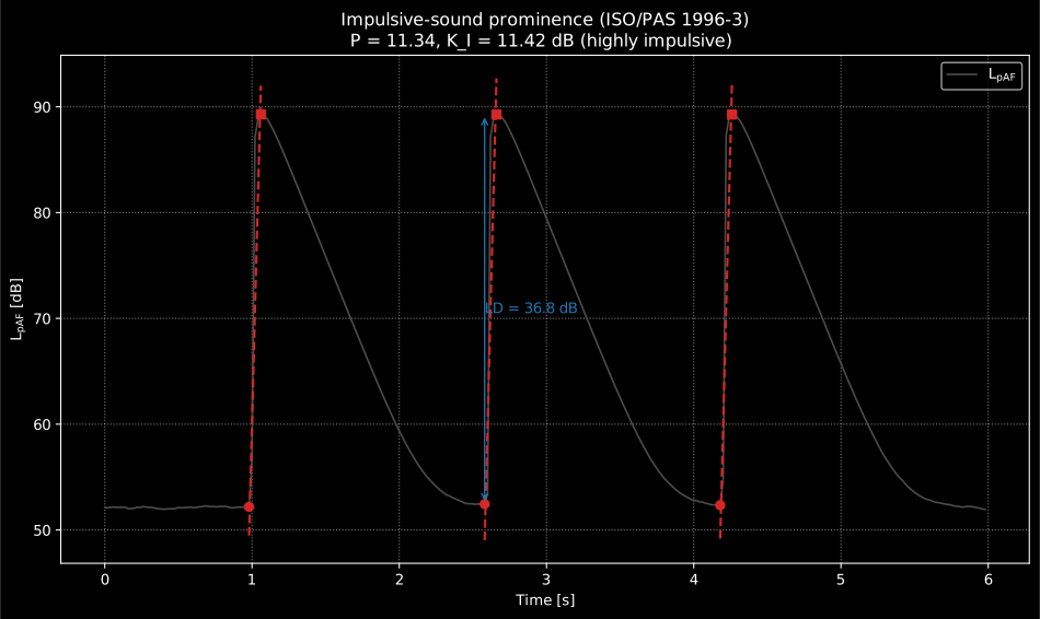
Two things are worth reading off the plot. The onset lines are the
least-squares fits over the detected rise, so a shallow fit on a visibly steep
edge means the level history was logged too coarsely to resolve it. And the
level difference is measured from the level just before the onset, not from
the long-term background, which is why a second strike arriving on the decay
tail of the first one scores a smaller LD than it appears to deserve.
Because the onset rate and level difference are level differences, the
adjustment is insensitive to the absolute calibration of the meter (clause 8);
only the reported LAeq and the adjusted LAeq depend on it. The scope of the
document states that the adjustment typically falls between 0,0 dB and 9,0 dB;
the formula itself is not capped, so a very sudden, loud impulse can exceed
that range. ImpulsiveSoundResult.plot() draws the LpAF history with the
detected onsets, the least-squares onset lines and the governing level
difference marked.
4. Where the method sits among the standards
Section titled “4. Where the method sits among the standards”Rating standards traditionally handle impulsiveness by category, not by measurement. ISO 1996-1:2016 (Table A.1) adds a fixed 5 dB when the source is regular impulsive and 12 dB when it is highly impulsive, and leaves the choice of category to the assessor’s judgement. NT ACOU 112 replaces that judgement with a measurement: the onset rate and level difference of the actual impulses produce a graduated that runs from 0 dB for barely perceptible onsets to about 18 dB for the most sudden, loud ones, crossing the two conventional figures on the way. The approach proved durable: the same onset-based prominence was later carried into ISO/PAS 1996-3:2022, which uses it to decide objectively whether a source counts as regular or highly impulsive in the ISO 1996-1 rating.
Two practical caveats when applying it. The onset is read from the
A-weighted, time-weighting-F level history, and the 125 ms time constant of
weighting F itself limits how fast a recorded level can rise: very short
impulses arrive already smoothed, so the level history must be logged at the
meter’s full output rate (not in coarse intervals); otherwise the onset rate,
and with it , is underestimated. And the method rates the prominence of the
impulses, not their energy: rides on top of the measured LAeq in the
rating level, it never replaces it.
5. Assessment report (.report())
Section titled “5. Assessment report (.report())”ImpulseProminenceResult.report(path) renders a one-page PDF fiche laid out
like an impulsive-sound assessment report of an environmental-noise laboratory,
following NT ACOU 112:2002 (carried into ISO/PAS 1996-3:2022): a
standard-basis line, an optional metadata header block (source/situation,
client, measurement position, instrumentation and date, with the 30-minute
assessment period always shown), a full-width per-impulse table (onset rate,
level difference, predicted prominence P and whether the onset qualifies as an
impulse) above the adjustment-curve plot KI(P) with the candidate
impulses marked, the boxed governing prominence P together with the derived
LAeq adjustment KI (Formula 2), an optional PASS/FAIL
verdict row and a prominence-category note, and a footer with the fixed
disclaimer.
It uses the same ReportMetadata container and rendering engine as the
ISO 532-1 loudness fiche;
a supplied requirement is read as the maximum acceptable governing prominence
P (a less prominent impulse passes). Rendering needs reportlab
(pip install phonometry[report]); only engine="reportlab" is supported. The
fiche renders in English by default; pass language="es" for a Spanish fiche
(translated fixed strings and a comma decimal separator), e.g.
res.report("impulse_fiche_es.pdf", language="es").
from phonometry import environmental, ReportMetadata
# The three-impulse pile-driving set from §1 (onset rate dB/s, level diff. dB).res = environmental.impulse_prominence([1200.0, 300.0, 60.0], [32.0, 18.0, 11.0])res.report(    "impulse_fiche.pdf",    metadata=ReportMetadata(        specimen="Pile-driving site, intermittent hammering",        measurement_standard="ISO 1996-2",        laboratory="Phonometry Reference Laboratory",        requirement=10.0,           # maximum acceptable governing prominence P    ),)                                   # governing P and the LAeq adjustment KI (dB)
The example fiche is regenerated with make reports and kept rendered in the
repository; click the preview to open the PDF.
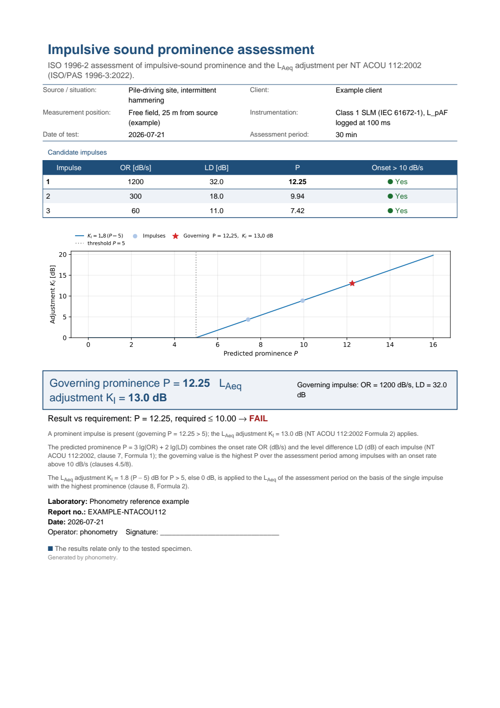
One-page impulsive-sound assessment fiche: a metadata header, a per-impulse table of the onset rate, level difference and predicted prominence P, the KI(P) adjustment-curve plot with the candidate impulses marked, the boxed governing prominence P = 12.25 with the LAeq adjustment KI = 13.0 dB (NT ACOU 112:2002 Formula 2) and a FAIL verdict against a maximum governing prominence of 10.
What this guide covers
Section titled “What this guide covers”Covered. NT ACOU 112:2002: the onset definition (clauses 4.5 to 4.7),
the predicted prominence P (clause 7, Formula 1), the graduated adjustment
KI (clause 8, Formula 2) and the rating level over a reference time
(clause 8, Note 1), through impulse_prominence, predicted_prominence,
impulse_adjustment and rating_level. ISO/PAS 1996-3:2022 is covered for
the objective measurement chain built on the same prominence formula: LpAF
sampling, onset detection and merging, and the least-squares onset rate and
level difference, through impulsive_sound_adjustment and detect_onsets.
Not covered. NT ACOU 112’s Note 4 (clause 7) records an older Nordic
guideline: a flat 5 dB adjustment based on subjective judgement, recommended
when KI > 3 for noise characteristic of working operations, offered as a
fallback where the graduated method cannot be applied. Only the graduated
KI of Formula 2 is implemented; the flat 5 dB alternative is not. ISO
1996-1’s Table A.1 category adjustments (5 dB regular, 12 dB highly
impulsive) are covered only as the assessor’s-judgement baseline that this
measurement replaces, not as a function of their own.
See also
Section titled “See also”- API reference:
environmental.impulse_prominence. - API reference:
environmental.impulsive_sound.
References
Section titled “References”- International Organization for Standardization. (2016). Acoustics — Description, measurement and assessment of environmental noise — Part 1: Basic quantities and assessment procedures (ISO 1996-1:2016). The rating framework and the Table A.1 category adjustments (5 dB regular, 12 dB highly impulsive) that the measured prominence calibrates against.
- International Organization for Standardization. (2022). Acoustics — Description, measurement and assessment of environmental noise — Part 3: Objective method for the measurement of prominence of impulsive sounds and for adjustment of LAeq (ISO/PAS 1996-3:2022). The ISO successor built on the NT ACOU 112 onset-rate prominence.
- Nordtest. (2002). Acoustics: Prominence of impulsive sounds and for adjustment of LAeq (NT ACOU 112:2002). The implemented method, freely downloadable from the Nordtest archive: the predicted prominence (clause 7, Formula 1), the adjustment to LAeq (clause 8, Formula 2) and the rating level (clause 8, Note 1), with the onset defined in clauses 4.5-4.7.