Porous and Multilayer Absorbers

Given a porous material’s flow resistivity (the quantity the flow rig measures) the classical equivalent-fluid models predict its complex characteristic impedance and wavenumber, and a transfer-matrix stack of layers (porous blankets, air gaps, perforated and microperforated panels, membranes) predicts the absorption coefficient of the whole construction before anything is built. This page covers the three porous models (Delany–Bazley, Miki, Johnson–Champoux–Allard), the multilayer solver, the resonant sheet layers of Maa and the random-incidence (Paris) integral. The measurement counterparts live in Acoustic Materials; rating the predicted spectrum lives in the same page’s ISO 11654 section.

1. Equivalent-fluid models of a porous material

A rigid-frame porous material behaves like an equivalent fluid with a complex characteristic impedance $Z_c$ and wavenumber $k$ (time convention $e^{+j\omega t}$, so a passive medium has $\mathrm{Im}(k)<0$).

Delany–Bazley (Mechel 2e Sect. G.11; Bies 5e Appendix D, Table D.1; Hopkins Eqs. 1.171–1.174) is the one-parameter power law in the absorber variable $X={\rho }_{0}f/\sigma$:

$$\frac{Z_c}{{\rho }_0{c}_0}=1+C_1{X}^{-C_2}-j{C}_3{X}^{-C_4},\frac{k}{k_0}=1+C_5{X}^{-C_6}-j{C}_7{X}^{-C_8},$$

with the classic rockwool/fibreglass coefficients $(0.0571,0.754,0.087,0.732,0.0978,0.700,0.189,0.595)$ and a stated fit range $0.01<X<1.0$ (porosity close to one). The library also ships the Table D.1 presets fitted to polyester ("garai_pompoli") and to foams ("dunn_davern", "wu"). Outside the fit range a PorousAbsorberWarning is raised and the extrapolated values are still returned; the classic failure is a negative real part of the layer input impedance at low frequency (Mechel Sect. G.12).

Miki (1990) refitted the same Delany–Bazley data under a passivity (positive-real) constraint, so the model stays physically well behaved below the fit range; it is the usual choice when a one-parameter model must be evaluated broadband.

Johnson–Champoux–Allard (JCA) is the five-parameter semi-phenomenological model (Cox & D’Antonio 3e Eqs. 6.19–6.25): flow resistivity $\sigma$, porosity $\varphi$, tortuosity ${\alpha }_{\infty }$ and the viscous/thermal characteristic lengths $\Lambda$, ${\Lambda }^{\prime }$ give the effective density and bulk modulus with the exact limits $j\omega {\rho }_e\to \sigma$ at DC, ${\rho }_e\to ({\alpha }_{\infty }{\rho }_0/\varphi )(1+(1-j){\delta }_v/\Lambda )$ at high frequency, and the isothermal-to-adiabatic transition in $K_e$.

import numpy as np
from phonometry import materials

f = np.geomspace(200.0, 4000.0, 200)
db = materials.delany_bazley(f, 20000.0)          # sigma in Pa s/m2
mk = materials.miki(f, 20000.0)
jca = materials.johnson_champoux_allard(
    f, 20000.0, porosity=0.98, tortuosity=1.0,
    viscous_length=8.7e-5, thermal_length=8.7e-5,
)
print(np.round(db.normalized_impedance[0], 3))    # (2.598-2.209j)
print(np.round(mk.normalized_impedance[0], 3))    # (2.286-1.965j)
print(np.round(jca.normalized_impedance[0], 3))   # (2.321-2.075j)

db.plot()   # normalised Zc and k components vs frequency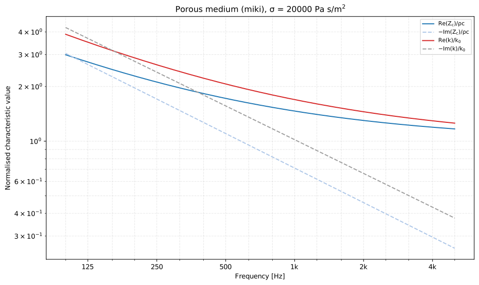

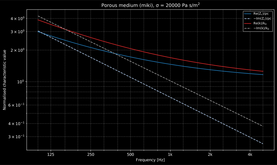
The classical presentation of an equivalent-fluid model (Cox & D’Antonio 3e, Figs. 6.19–6.20): at low frequency the viscous forces dominate and the material looks stiff and lossy (all four components large); as frequency rises the components fall towards the free-air limits $Z_c\to {\rho }_0{c}_0$ and $k\to k_0$, so a thin layer only works where its thickness is a fair fraction of the wavelength inside the material.

Show the code for this figure

import matplotlib.pyplot as plt
import numpy as np
from phonometry import materials

f = np.geomspace(100.0, 5000.0, 260)
mk = materials.miki(f, 20000.0)          # sigma = 20 kPa s/m^2

# One line: normalised Zc and k components on a log-log grid.
mk.plot()
plt.show()

# By hand, from the result's fields:
fig, ax = plt.subplots()
ax.loglog(f, mk.normalized_impedance.real, label="Re(Zc)/rho c")
ax.loglog(f, -mk.normalized_impedance.imag, "--", label="-Im(Zc)/rho c")
ax.loglog(f, mk.normalized_wavenumber.real, label="Re(k)/k0")
ax.loglog(f, -mk.normalized_wavenumber.imag, "--", label="-Im(k)/k0")
ax.set(xlabel="Frequency [Hz]", ylabel="Normalised characteristic value")
ax.legend()
plt.show()

The three models agree closely over the Delany–Bazley fit range (Cox & D’Antonio Figs. 6.19–6.21 make the same comparison); JCA extends the prediction physically outside it. A PorousMediumResult built from measured data (for example the $Z_c$, $k$ recovered by the ASTM E2611 transfer-matrix reduction) plugs into the layer solver exactly like a modelled one.

2. Multilayer prediction by transfer matrices

Each fluid layer of thickness $d$ contributes the chain matrix (Cox & D’Antonio Eq. 2.29; equivalently the impedance recursion of Bies Eq. D.95 and Mechel Sect. D.4)

$${\left[\begin{array}{c}p\\ u\end{array}\right]}_{\text{front}}=\left[\begin{array}{cc}\cos (k_{x}d)& j{Z}_x\sin (k_{x}d)\\ j\sin (k_{x}d)/Z_x& \cos (k_{x}d)\end{array}\right]{\left[\begin{array}{c}p\\ u\end{array}\right]}_{\text{back}},$$

with the in-depth wavenumber $k_x=\sqrt{k^2-k_0^2{\sin }^2\theta }$ from Snell’s law and $Z_x=Z_{c}k/k_x$. Thin resonant sheets enter as series impedances $[[1,z],[0,1]]$. Closing the chain with a rigid wall (or free air, or any impedance) gives the surface impedance, the reflection factor $R(\theta )$ and $\alpha (\theta )=1-|R{|}^2$. A single hard-backed porous layer reduces to the textbook closed form $Z_s=-j{Z}_c\cot (kd)$ (Mechel Sect. D.3, Eq. 1).

import numpy as np
from phonometry import materials

f = np.geomspace(200.0, 4000.0, 300)
med = materials.miki(f, 20000.0)
res = materials.layered_absorber(f, [materials.PorousLayer(0.05, med)])
i = np.argmin(np.abs(f - 1000.0))
print(round(res.absorption[i], 3))               # 0.937 at 1 kHz

res.plot()   # alpha(f) with |R| overlaid

The solver evaluates the physical quantities through a numerically robust admittance recursion (immune to the $e^{|\mathrm{Im}(k_x)|d}$ overflow of raw matrix entries for extremely attenuating layers) and still exposes the full chain matrix (reciprocal by construction, $\det T=1$) in transfer_matrix, ready for the ASTM E2611 machinery (TransferMatrix).

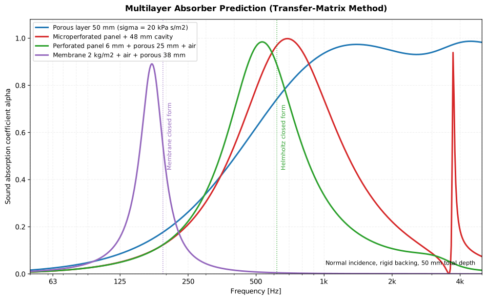
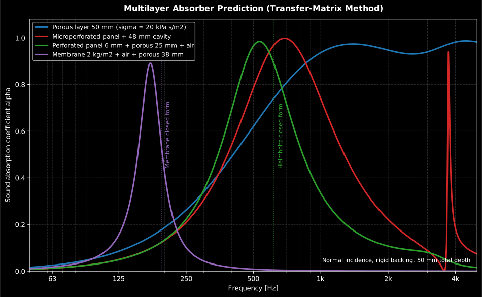
Four constructions, one 50 mm budget: the porous layer works broadband but fades at low frequency; the microperforated, perforated and membrane designs trade bandwidth for a resonant peak placed ever lower. The dotted lines are the shallow-cavity closed forms; the full model sits below them because the viscous plug mass and the finite cavity depth are not negligible.

Show the code for this figure

import matplotlib.pyplot as plt
import numpy as np
from phonometry import materials as m

f = np.geomspace(50.0, 5000.0, 500)
med = m.miki(f, 20000.0)
med_light = m.miki(f, 10000.0)
designs = {
    "Porous 50 mm": [m.PorousLayer(0.05, med)],
    "MPP + cavity": [m.MicroperforatedPlateLayer(0.5e-3, 0.15e-3, 0.008),
                     m.AirLayer(0.048)],
    "Perforated + porous": [m.PerforatedPlateLayer(0.006, 0.0025, 0.05),
                            m.PorousLayer(0.025, med), m.AirLayer(0.019)],
    "Membrane + porous": [m.MembraneLayer(2.0), m.AirLayer(0.01),
                          m.PorousLayer(0.038, med_light)],
}
fig, ax = plt.subplots()
for label, layers in designs.items():
    ax.semilogx(f, m.layered_absorber(f, layers).absorption, label=label)
ax.set(xlabel="Frequency [Hz]", ylabel="Absorption coefficient")
ax.legend()
plt.show()

Behind every one of those curves there is a plain layer list, read front to back in the order the incident wave meets it. plot_absorber_stack draws that list to scale before any physics runs, and a solved result retains its layers, so materials.layered_absorber(f, layers).plot_geometry() draws the same cross-section from the result itself.

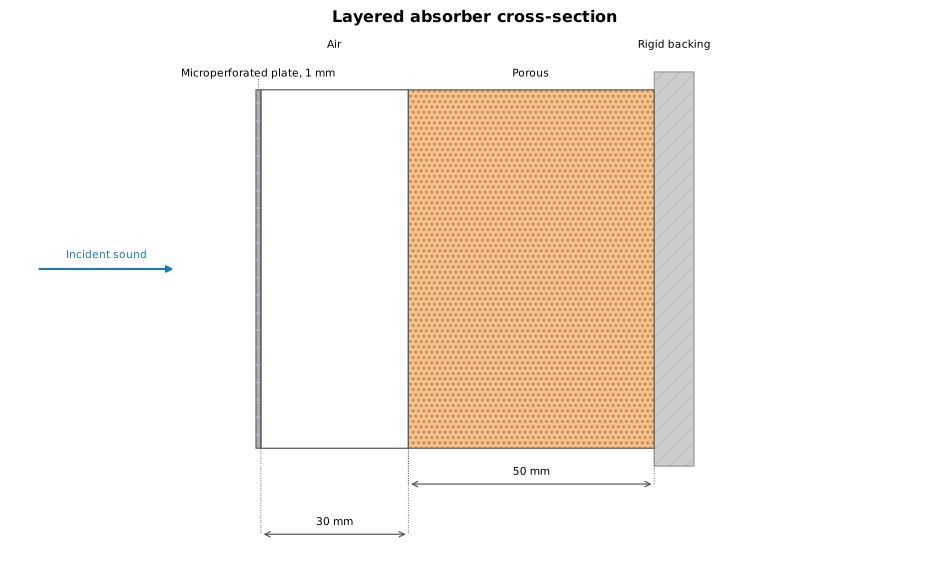
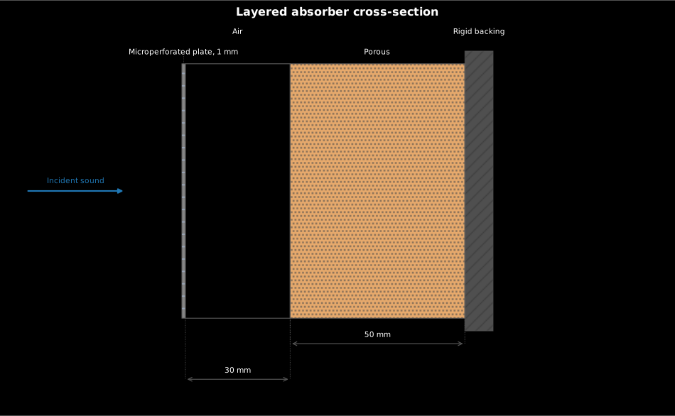
The layer list as the wave meets it: microperforated plate, air cavity, porous layer, rigid backing. Drawing the stack to scale before computing anything catches the classic metres-versus-millimetres slip in a thickness at a glance.

Show the code for this figure

import matplotlib.pyplot as plt
import numpy as np
from phonometry import materials

f = np.linspace(200.0, 4000.0, 100)
layers = [
    materials.MicroperforatedPlateLayer(0.001, 0.0002, 0.01),
    materials.AirLayer(0.03),
    materials.PorousLayer(0.05, materials.miki(f, 20000.0)),
]

# The free function draws any layer list; a solved result retains its
# layers, so this draws the same cross-section:
#   materials.layered_absorber(f, layers).plot_geometry()
materials.plot_absorber_stack(layers)
plt.show()

3. Resonant sheets: perforated, microperforated, membrane

Perforated panel. The air plugs in the holes are the mass of a Helmholtz resonator: $m=({\rho }_0/\epsilon )[t+2\delta a+\sqrt{8\nu /\omega }(1+t/2a)]$ with the open area $\epsilon$, the end-correction factor $\delta$ per orifice end and the visco-thermal resistance $r=({\rho }_0/\epsilon )\sqrt{8\nu \omega }(1+t/2a)$ (Cox & D’Antonio Eqs. 7.6/7.12). The default end correction is the Fok-function interaction fit $\delta =0.85(1-1.47\sqrt{\epsilon }+0.47{\epsilon }^{3/2})$ (Table 7.1), valid for any open area. For a shallow cavity the resonance is $f_0=(c_0/2\pi )\sqrt{\epsilon /(t^{\prime }d)}$ (Eq. 7.4).

Microperforated panel (MPP). With submillimetre holes the viscous boundary layer fills the orifice and the panel absorbs without any porous material. The library implements Maa’s exact short-tube impedance (Maa 1998, Eq. 2),

$$z_1=j\omega {\rho }_{0}t{\left[1-\frac{2}{x\sqrt{-j}}\frac{J_1(x\sqrt{-j})}{J_0(x\sqrt{-j})}\right]}^{-1},x=a\sqrt{{\rho }_0\omega /\eta },$$

plus the Eq. 5 end corrections (surface resistance $\frac{1}{2}\sqrt{2\omega {\rho }_0\eta }$ and piston reactance $0.85d$ total), divided by the open area. The perforate constant $x$ (proportional to the hole radius over the viscous boundary-layer thickness) governs everything: at the resonance ${\omega }_{0}m=\cot ({\omega }_{0}D/c_0)$ the peak absorption is $4r/(1+r{)}^2$ and the half-absorption bandwidth is $f_2/f_1=\pi /\mathrm{arccot}(1+r)-1$ (Maa Eqs. 9–21, Table I).

import numpy as np
from phonometry import materials

# Maa (1998) Fig. 5: d = t = 0.2 mm, holes every 2.5 mm, cavity 6 cm.
eps = (np.pi / 4.0) * (0.2 / 2.5) ** 2
f = np.linspace(100.0, 4000.0, 2000)
res = materials.layered_absorber(
    f, [materials.MicroperforatedPlateLayer(0.2e-3, 0.1e-3, eps),
        materials.AirLayer(0.06)],
)
i = np.argmax(res.absorption)
print(f"peak alpha = {res.absorption[i]:.2f} at {f[i]:.0f} Hz")
# peak alpha = 0.96 at 677 Hz
res.plot()   # alpha(f) with |R| overlaid: the resonant MPP peak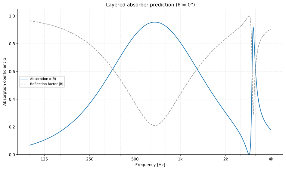

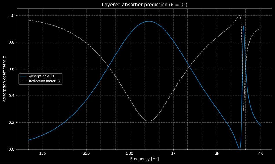
Maa’s own Fig. 5 design, no porous material anywhere: the viscous losses in the submillimetre holes damp the panel-cavity resonance into a broad absorption peak. The narrow feature near 2.9 kHz is the half-wave cavity resonance, where the cavity presents a pressure node to the panel and the absorption collapses before the next resonance restores it.

Show the code for this figure

import matplotlib.pyplot as plt
import numpy as np
from phonometry import materials

# Maa (1998) Fig. 5: d = t = 0.2 mm, holes every 2.5 mm, cavity 6 cm.
eps = (np.pi / 4.0) * (0.2 / 2.5) ** 2
f = np.linspace(100.0, 4000.0, 1200)
res = materials.layered_absorber(
    f, [materials.MicroperforatedPlateLayer(0.2e-3, 0.1e-3, eps),
        materials.AirLayer(0.06)],
)

# One line: alpha(f) with |R| overlaid.
res.plot()
plt.show()

# By hand, from the result's fields:
fig, ax = plt.subplots()
ax.semilogx(f, res.absorption, label="Absorption alpha")
ax.semilogx(f, np.abs(res.reflection), "--", label="Reflection factor |R|")
ax.set(xlabel="Frequency [Hz]", ylabel="Coefficient")
ax.legend()
plt.show()

Membrane. A limp impervious sheet is the surface mass $z=j\omega m$ (Cox Eq. 7.14; Bies Eq. D.96); over a cavity it resonates at the classical $f_0\approx 60/\sqrt{md}$ (adiabatic; $\approx 50/\sqrt{md}$ when the cavity is porous-filled and isothermal, Cox Eqs. 7.9/7.10). The closed forms are exposed as helmholtz_resonance_frequency and membrane_resonance_frequency; the full frequency response comes from the same layer stack.

4. Oblique and random incidence

layered_absorber(..., angle=theta) evaluates the full bulk-reacting stack at any polar angle; sheets are locally reacting (angle-independent), fluid layers refract per Snell’s law; for an MPP over a cavity this reproduces Maa’s oblique closed form (Eq. 23) exactly. The random-incidence coefficient is the Paris integral (Mechel Sect. D.5, Eq. 9)

$${\alpha }_{dif}=\frac{2}{{\sin }^2{\theta }_{lim}}{\int }_0^{{\theta }_{lim}}\alpha (\theta )\cos \theta \sin \theta \mathrm{d}\theta ,$$

evaluated by Gauss–Legendre quadrature in diffuse_field_absorption (angle_limit defaults to 90°; truncations at 75–87° are in use). For a locally reacting surface with known normalised impedance the integral has the closed form of Mechel Eq. 10, exposed as statistical_absorption; its maximum over all passive impedances is the published 0.951 (at $z\approx 1.57$).

import numpy as np
from phonometry import materials

f = np.array([250.0, 500.0, 1000.0, 2000.0])
med = materials.miki(f, 20000.0)
layers = [materials.PorousLayer(0.05, med)]
normal = materials.layered_absorber(f, layers)
diffuse = materials.diffuse_field_absorption(f, layers)
print(np.round(normal.absorption, 2))    # [0.26 0.62 0.94 0.95]
print(np.round(diffuse.absorption, 2))   # [0.37 0.68 0.9  0.95]
diffuse.plot()   # alpha_dif(f); overlay normal.absorption to compare

print(round(float(materials.statistical_absorption(1.567 + 0j)), 3))  # 0.951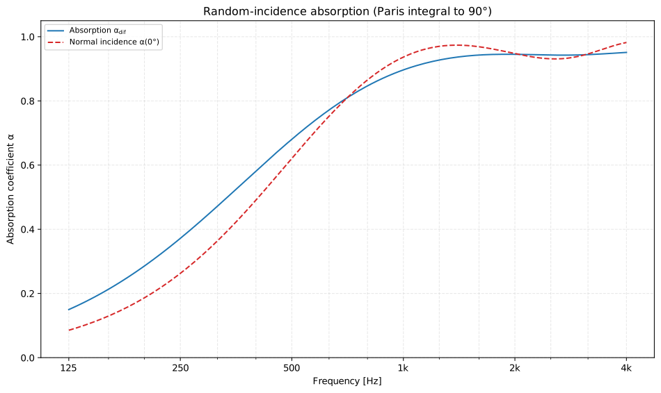

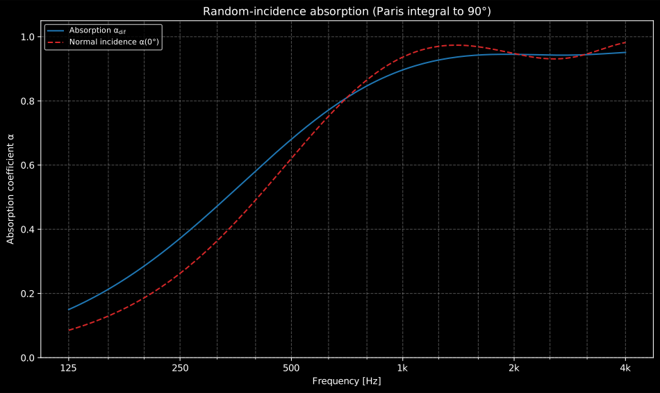
Why the reverberation room reads higher than the tube: the Paris integral weights the oblique angles, whose waves travel a longer path inside the layer, so ${\alpha }_{dif}$ exceeds the normal-incidence $\alpha (0°)$ exactly where the layer is thin against the wavelength. This is the model-side counterpart of the tube-versus-reverberation-room discussion of Acoustic Materials.

Show the code for this figure

import matplotlib.pyplot as plt
import numpy as np
from phonometry import materials

f = np.geomspace(125.0, 4000.0, 200)
layers = [materials.PorousLayer(0.05, materials.miki(f, 20000.0))]
normal = materials.layered_absorber(f, layers)
diffuse = materials.diffuse_field_absorption(f, layers)

# One line, then the normal-incidence overlay on the same axes:
ax = diffuse.plot()
ax.plot(f, normal.absorption, "--", label="Normal incidence alpha(0)")
ax.legend()
plt.show()

5. Slow-sound slit panels with Helmholtz resonators

A rigid panel perforated by a periodic array of thin closed slits, each slit loaded on its upper wall by an array of Helmholtz resonators, is a locally reacting, deep-subwavelength absorber (Jiménez et al. 2017). The resonators slow the sound inside the slit, pulling the slit resonance far below the quarter-wavelength frequency, so a panel a few centimetres deep resonates in the low hundreds of hertz. The visco-thermal losses in the sub-millimetre slit and in the resonator necks are what make perfect absorption possible: when the intrinsic loss exactly balances the leakage of the structure the reflection zero lands on the real-frequency axis and $\alpha =1$ (critical coupling).

The panel transfer matrix is the chain $T=M_{\Delta l}{\prod }_n(M_s{M}_{HR}^{(n)}{M}_s)$ of half-lattice slit steps (with slit characteristic impedance $Z_s=\sqrt{{\kappa }_s{\rho }_s}/S_s$), resonators as shunt point scatterers $[[1,0],[1/Z_{HR},1]]$, and a slit-radiation end correction. The rigidly-backed reflection factor is $R=(T_{11}\cos \theta -Z_0{T}_{21})/(T_{11}\cos \theta +Z_0{T}_{21})$ with $Z_0={\rho }_0{c}_0/S_0$ and $\alpha =1-|R{|}^2$. The slit uses the narrow-channel visco-thermal parameters and the square necks and cavities the rectangular-duct series of Stinson (1991).

critical_coupling_design inverts the model: given a target frequency and angle it tunes the cavity length (which sets the resonance) and the slit height (which sets the loss) so both matching conditions $\mathrm{Re}(Z)\cos \theta =Z_0$ and $\mathrm{Im}(Z)=0$ hold, placing the reflection zero on the real axis. The returned geometry then gives $\alpha \approx 1$ at the design frequency.

import numpy as np
from phonometry import (
    HelmholtzResonator, critical_coupling_design, slit_helmholtz_absorber,
)

base = HelmholtzResonator(
    neck_length=1.0e-3, neck_side=3.0e-3,
    cavity_length=30.0e-3, cavity_side=27.0e-3,
)
design = critical_coupling_design(
    300.0, base, lattice_step=3.0e-2, period=5.0e-2,
)
print(round(design.absorption, 4))          # ~1.0 (perfect absorption)
print(round(design.slit_height * 1e3, 3))    # solved slit height, mm

f = np.linspace(150.0, 500.0, 700)
res = slit_helmholtz_absorber(
    f, design.resonator, slit_height=design.slit_height,
    lattice_step=3.0e-2, period=5.0e-2,
)
res.plot()   # alpha(f) with |R| overlaid; peak = 1 at 300 Hz

The solved geometry is worth a look before the absorption curve. The resonator draws itself with .plot() and the panel result with .plot_geometry(), both dimensioned and to scale.

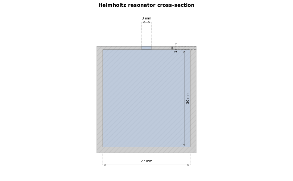
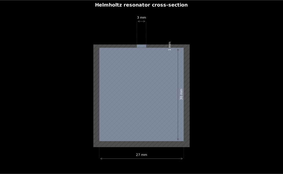
The four numbers that define the resonator: the neck side and length set the moving mass and most of the loss, the cavity side and length set the stiffness. critical_coupling_design keeps this cross-section and retunes the cavity length to place the resonance.

Show the code for this figure

import matplotlib.pyplot as plt
from phonometry import HelmholtzResonator

resonator = HelmholtzResonator(
    neck_length=1.0e-3, neck_side=3.0e-3,
    cavity_length=30.0e-3, cavity_side=27.0e-3,
)
resonator.plot()   # dimensioned cross-section, to scale
plt.show()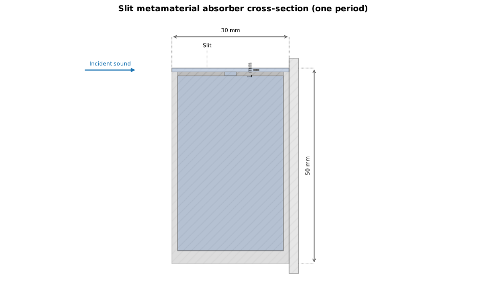

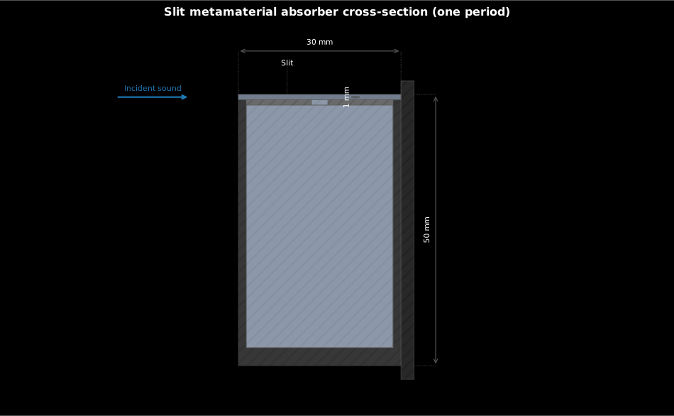
One period of the solved design, to scale: the whole panel is 30 mm deep, $\lambda /38$ at 300 Hz, and the sub-millimetre slit that does all the absorbing is barely visible. That is exactly the point of the slow-sound mechanism.

Show the code for this figure

import matplotlib.pyplot as plt
from phonometry import HelmholtzResonator, critical_coupling_design, materials

base = HelmholtzResonator(
    neck_length=1.0e-3, neck_side=3.0e-3,
    cavity_length=30.0e-3, cavity_side=27.0e-3,
)
design = critical_coupling_design(
    300.0, base, lattice_step=3.0e-2, period=5.0e-2,
)

# The free function draws any resonator list; a slit_helmholtz_absorber
# result retains its geometry, so res.plot_geometry() draws the same period.
materials.plot_slit_absorber_geometry(
    [design.resonator], slit_height=design.slit_height,
    lattice_step=3.0e-2, period=5.0e-2,
)
plt.show()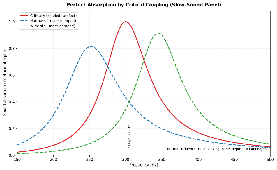

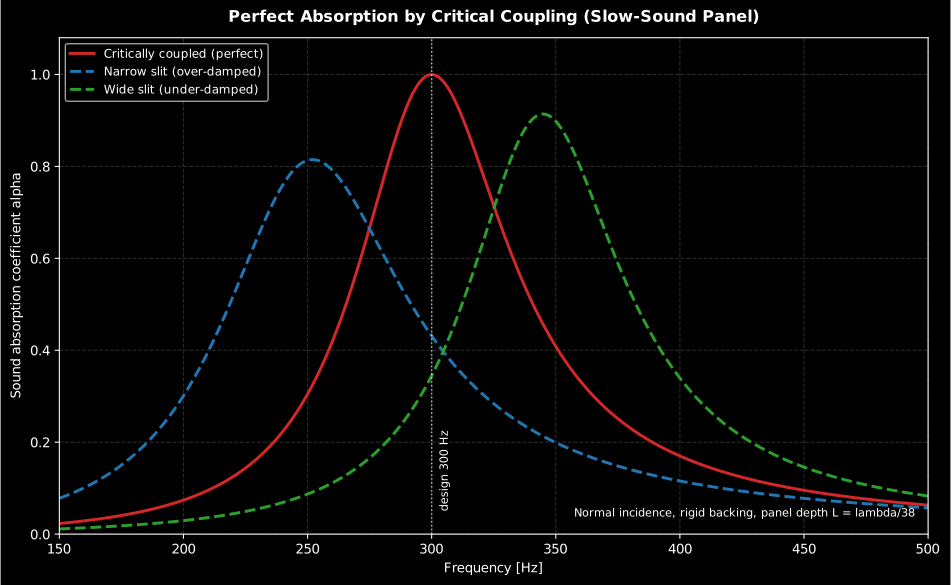
One resonator, one slit, one loss-versus-leakage balance. The critically coupled design reaches $\alpha =1$ at 300 Hz in a panel only $\lambda /38$ deep; narrowing the slit over-damps the resonance and widening it under-damps it, both dropping the peak below one.

Show the code for this figure

import matplotlib.pyplot as plt
import numpy as np
from phonometry import (
    HelmholtzResonator, critical_coupling_design, slit_helmholtz_absorber,
)

a, d, f0 = 3.0e-2, 5.0e-2, 300.0
base = HelmholtzResonator(1.0e-3, 3.0e-3, 30.0e-3, 27.0e-3)
design = critical_coupling_design(f0, base, lattice_step=a, period=d)
h0 = design.slit_height

f = np.linspace(150.0, 500.0, 700)
fig, ax = plt.subplots()
for factor, label in [(1.0, "critically coupled"),
                      (0.6, "narrow slit"), (1.7, "wide slit")]:
    res = slit_helmholtz_absorber(
        f, design.resonator, slit_height=factor * h0,
        lattice_step=a, period=d,
    )
    ax.plot(f, res.absorption, label=label)
ax.set(xlabel="Frequency [Hz]", ylabel="Absorption coefficient")
ax.legend()
plt.show()

Practical notes

Fit ranges. Delany–Bazley warns (and extrapolates) outside $0.01<X<1$ and Miki outside $0.01<f/\sigma <1$; treat sub-range values as qualitative. JCA needs four extra parameters but behaves physically everywhere; with $\Lambda ={\Lambda }^{\prime }=\sqrt{8{\alpha }_{\infty }\eta /(\varphi \sigma )}$ and ${\alpha }_{\infty }=1$ it tracks Delany–Bazley over the fit range.

Local vs. bulk reaction. The layer solver is bulk-reacting (sound refracts and travels inside the layers). statistical_absorption assumes local reaction, a good approximation for high flow resistivity, partitioned cavities or thin resonant facings; for thick, light porous layers integrate the bulk model with diffuse_field_absorption instead (Mechel Sect. D.6).

Where the numbers were checked. No standard governs these prediction models; they are textbook and journal methods implemented clean-room from the sources in the references below. The models are pinned digit-exact to the printed coefficient tables (Bies Table D.1, Miki Eqs. 30–34), the solver to the closed forms above and to the TransferMatrix recovery of the impedance-tube page, the MPP to Maa’s own approximation (stated ~6 % agreement with the exact Eq. 2), design example and Table I, and the Paris integral to its locally reacting closed form. The slow-sound slit + Helmholtz-resonator model is pinned to its exact analytic anchors: the critical-coupling design reaches $\alpha =1$ at the design frequency, the slit and square-duct effective densities reduce to the Poiseuille flow resistivities $12\eta /h^2$ and $28.454\eta /w^2$ as $\omega \to 0$, and the effective parameters tend to ${\rho }_0$, ${\kappa }_0$ as the boundary layers vanish. Five misprints found in the sources during this work are recorded in the errata registry.

What this guide covers

Covered. No standard governs these prediction models: they are textbook and journal methods implemented clean-room from Mechel, Bies, Cox & D’Antonio, Miki (1990), Maa (1998), Johnson, Koplik & Dashen (1987) and Jiménez et al. (2016/2017), the sources listed above. That covers the equivalent-fluid porous models (delany_bazley, miki, johnson_champoux_allard), the transfer-matrix multilayer solver (layered_absorber with PorousLayer, PerforatedPlateLayer, MicroperforatedPlateLayer and MembraneLayer), the Paris-integral random-incidence coefficients (diffuse_field_absorption, statistical_absorption) and the critically-coupled slit and Helmholtz-resonator absorber (slit_helmholtz_absorber, critical_coupling_design).

Not covered. Cox & D’Antonio’s book covers diffusers as well as absorbers, but this guide only implements the absorber half of it. Schroeder phase-grating diffuser prediction lives in a separate module (materials.diffuser_design), documented in Surface Scattering, Diffusion and In-situ Absorption.

See also

• Acoustic Materials: the measurement standards these prediction models connect to, namely ISO 9053-1/-2 (flow resistivity), ISO 10534-1/-2 and ASTM E2611 (impedance tube), and ISO 354 / ISO 11654 (random-incidence absorption and rating).

References

• Attenborough, K., & Van Renterghem, T. (2021). Predicting outdoor sound (2nd ed.). CRC Press. https://doi.org/10.1201/9780429470806Chapter 5: ground-impedance models, including the JCA family.
• Bies, D. A., Hansen, C. H., & Howard, C. Q. (2017). Engineering noise control (5th ed.). CRC Press. https://doi.org/10.1201/9781351228152Appendix D: porous-material properties, Table D.1 coefficient sets and the layered-construction recursions D.91-D.99.
• Cox, T. J., & D'Antonio, P. (2017). Acoustic absorbers and diffusers: Theory, design and application (3rd ed.). CRC Press. https://doi.org/10.1201/9781315369211Transfer-matrix modelling (Sect. 2.6), porous models (Sect. 6.5) and resonant-absorber design equations (Sects. 7.3/7.5).
• Delany, M. E., & Bazley, E. N. (1970). Acoustical properties of fibrous absorbent materials. Applied Acoustics, 3(2), 105-116. https://doi.org/10.1016/0003-682X(70)90031-9The original empirical relations and their stated validity.
• Hopkins, C. (2007). Sound insulation. Butterworth-Heinemann. https://doi.org/10.4324/9780080550473Section 1.3.2.2: the equivalent-gas model and the Delany-Bazley SI form.
• Jimenez, N., Groby, J.-P., Pagneux, V., & Romero-Garcia, V. (2017). Iridescent perfect absorption in critically-coupled acoustic metamaterials using the transfer matrix method. Applied Sciences, 7(6), 618. https://doi.org/10.3390/app7060618The slit + Helmholtz-resonator transfer-matrix model and the critical-coupling (perfect-absorption) condition implemented in slit_helmholtz_absorber.
• Jimenez, N., Huang, W., Romero-Garcia, V., Pagneux, V., & Groby, J.-P. (2016). Ultra-thin metamaterial for perfect and quasi-omnidirectional sound absorption. Applied Physics Letters, 109(12), 121902. https://doi.org/10.1063/1.4962328The resonator impedance (Eq. A23), its radiation end corrections (Eqs. A24-A27) and the worked slow-sound examples.
• Johnson, D. L., Koplik, J., & Dashen, R. (1987). Theory of dynamic permeability and tortuosity in fluid-saturated porous media. Journal of Fluid Mechanics, 176, 379-402. https://doi.org/10.1017/S0022112087000727The dynamic-tortuosity model behind the JCA effective density.
• Maa, D.-Y. (1998). Potential of microperforated panel absorber. The Journal of the Acoustical Society of America, 104(5), 2861-2866. https://doi.org/10.1121/1.423870The exact MPP impedance (Eq. 2), end corrections, design formulas and the Fig. 5 example pinned in the tests.
• Mechel, F. P. (Ed.). (2008). Formulas of acoustics (2nd ed.). Springer. https://doi.org/10.1007/978-3-540-76833-3Sections D.3-D.6 (layer reflection, multilayer scheme, diffuse-field integrals) and G.11 (empirical porous relations).
• Miki, Y. (1990). Acoustical properties of porous materials — Modifications of Delany-Bazley models. Journal of the Acoustical Society of Japan (E), 11(1), 19-24. https://doi.org/10.1250/ast.11.19The positive-real regression implemented in miki.
• Stinson, M. R. (1991). The propagation of plane sound waves in narrow and wide circular tubes, and generalization to uniform tubes of arbitrary cross-sectional shape. The Journal of the Acoustical Society of America, 89(2), 550-558. https://doi.org/10.1121/1.400379The visco-thermal effective density and bulk modulus of the slit and of the square necks and cavities.