Image Sources and the Steady-State Room Field

By José M. Requena Plens · Published Jul 19, 2026, updated Jul 26, 2026

Key references: Kuttruff 2016 Vorländer 2020 Allen & Berkley 1979 Bies et al. 2017

Two classical models predict the sound field in a rectangular room before it is ever built. The image-source model gives the deterministic early reflection pattern — the whole room impulse response as a sum of mirror images of the source — while the steady-state model gives the statistical level a source of known power settles to, split into a direct and a reverberant field. This page covers both in phonometry.room: the first complements the measured impulse response of the Room Acoustics guide with a synthetic one, and the second complements the single decay rate of the Reverberation-time prediction guide with a level-versus-distance prediction, bridging the sound power of a source and the level it produces indoors.

1. Image-source room impulse response

A rigid or absorbing rectangular room — a shoebox — reflects a point source in its six walls, and each reflection is exactly the free-field sound of a mirror image of the source. Mirroring a coordinate in a wall ( $S_{n} = S - 2 d n$ ) turns the source into a regular lattice of images, and the room impulse response is the direct sound plus one delayed, attenuated impulse per image,

g (t) = n \sum A_{n} δ (t - t_{n}), A_{n} = \frac{1}{4 π r _{n}} e^{- m r_{n} /2} walls \prod R_{w}^{k_{w, n}}, t_{n} = \frac{r _{n}}{c} .

Each image at distance $r_{n}$ from the receiver arrives at $t_{n} = r_{n} / c$ with an amplitude built from the $1/ (4 π r_{n})$ spherical spreading, the product of the wall pressure reflection factors $R_{w} = 1 - α_{w}$ each raised to the number of reflections $k_{w, n}$ that image made off wall $w$ , and the air pressure loss $e^{- m r_{n} /2}$ over the path ( $m$ the intensity attenuation coefficient, so intensity falls as $e^{- m r}$ ). A shoebox has exactly $\frac{2}{3} (2 i_{0}^{3} + 3 i_{0}^{2} + 4 i_{0})$ audible images up to reflection order $i_{0}$ (1560 at order 10), and the reflection density grows as $d N / d t = 4 π c^{3} t^{2} / V$ .

import numpy as np
from phonometry import room

# A 7 x 5 x 3 m room, source and receiver off-centre.
res = room.image_source_rir(
    dimensions=(7.0, 5.0, 3.0),
    source=(2.0, 1.6, 1.5),
    receiver=(5.2, 3.4, 1.7),
    absorption=0.12,          # uniform wall absorption (scalar)
    fs=48000,
    max_order=12,
)

print(res.ir.shape)                          # (n_samples,) broadband RIR
print(round(res.direct_time * 1000, 2))      # direct-sound arrival, ms
print(res.times.size == room.audible_image_count(12) + 1)   # images + source

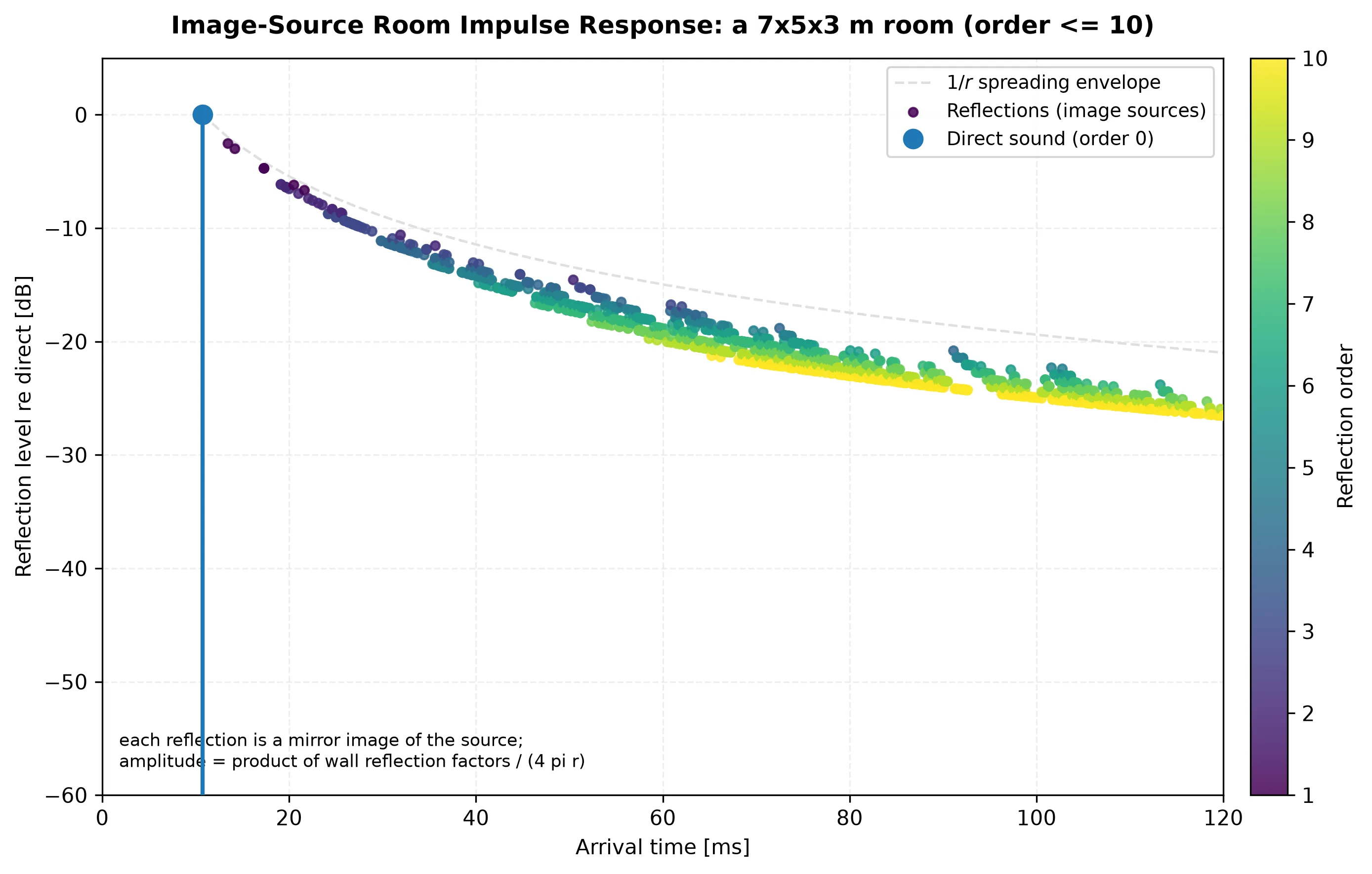
res.plot()   # the reflectogram of the figure below

# The synthetic RIR flows straight into the ISO 3382 decay analysis.
params = room.room_parameters(res.ir, res.fs, limits=None)
print(bool(params.t30_valid[0]))             # True: the decay window is usable
# T30 rises toward the Eyring estimate as max_order grows (see below); at a low
# order the specular tail is truncated, so treat this as an order-limited value.
print(round(float(params.t30[0]), 2))        # reverberation time, s

image_source_rir returns an ImageSourceResult. Its ir is the sampled RIR (a 1D array broadband, or one row per octave band for per-band absorption), while the exact sub-sample reflection table stays in times, distances, orders, amplitudes and image_positions — so the geometry is exact regardless of the sample rate. The direct sound and the individual early reflections are geometric quantities good to machine precision.

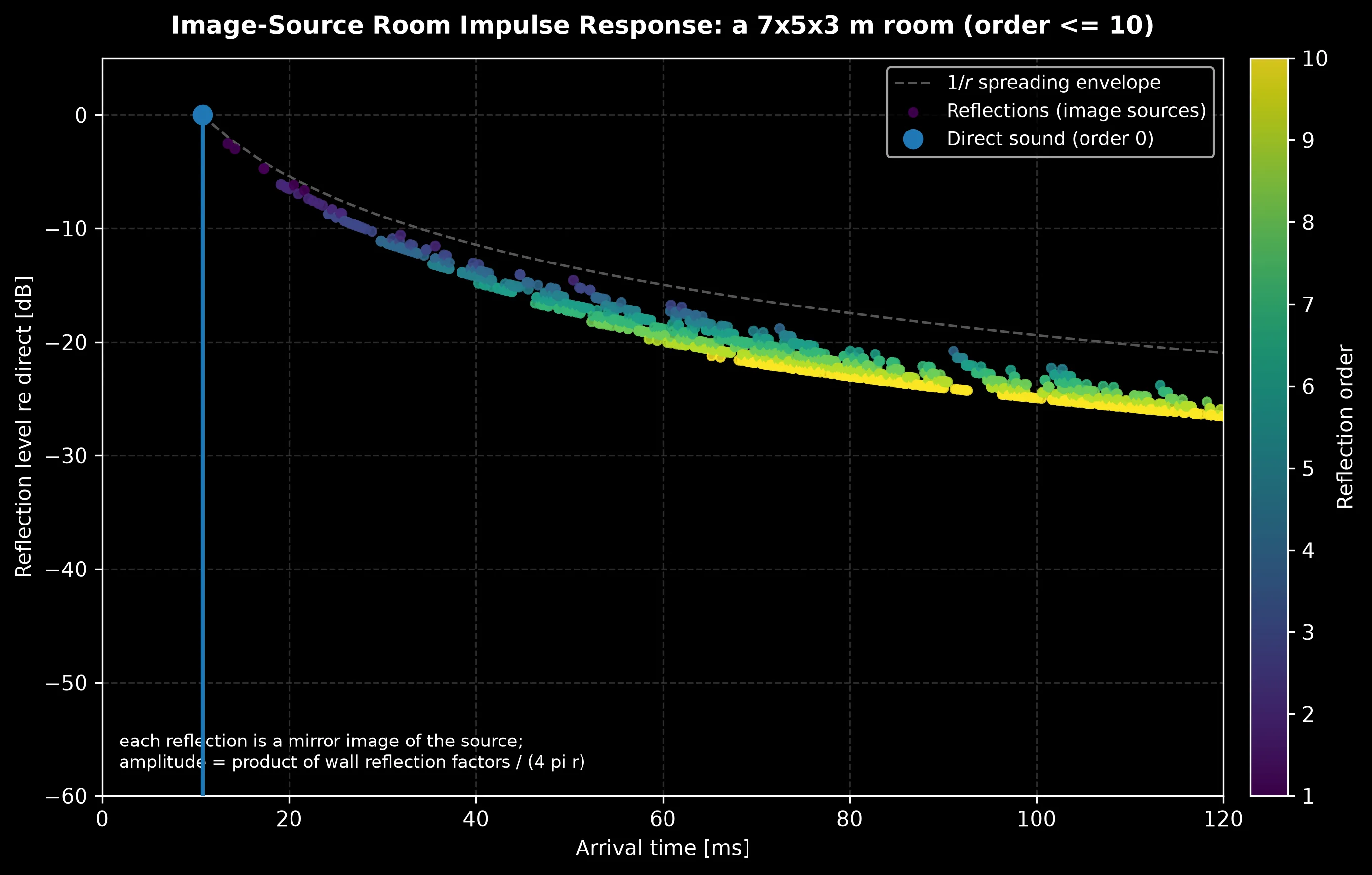
The reflectogram below shows the whole pattern: the direct sound at 0 dB, then the reflection cloud coloured by reflection order decaying under the $1/ r$ spreading envelope. Order-1 reflections (the six walls) sit just below the direct sound; higher orders arrive later, denser and weaker.

Image-source reflectogram of a 7 by 5 by 3 metre room: the direct sound at 0 dB followed by a cloud of reflections coloured by reflection order that decays under the 1/r spreading envelope, denser and weaker with time

Show the code for this figure

import matplotlib.pyplot as plt
import numpy as np
from phonometry import room

res = room.image_source_rir((7.0, 5.0, 3.0), (2.0, 1.6, 1.5),
                            (5.2, 3.4, 1.7), 0.12, fs=48000, max_order=10)

# One line: the reflectogram (level in dB re direct vs arrival time, by order).
res.plot()
plt.show()

# By hand: scatter the reflection amplitudes coloured by order.
t_ms = np.asarray(res.times) * 1e3
amp = np.asarray(res.amplitudes)
level = 20 * np.log10(np.abs(amp) / np.max(np.abs(amp)))
order = np.asarray(res.orders)
fig, ax = plt.subplots()
sc = ax.scatter(t_ms[order > 0], level[order > 0], c=order[order > 0],
                cmap="viridis", s=18)
ax.stem([t_ms[order == 0][0]], [0.0])         # direct sound
fig.colorbar(sc, label="Reflection order")
ax.set_xlabel("Arrival time [ms]"); ax.set_ylabel("Level re direct [dB]")
ax.set_xlim(0, 120); ax.set_ylim(-60, 5)
plt.show()

Per band, per wall and with air. Pass per-band coefficients (a (6, n_bands) per-wall array, a per-band vector or a frequencies list) to synthesise one decay per octave band; a length-6 vector sets each wall separately (order x0, xL, y0, yL, z0, zL); and air_attenuation (the intensity coefficient m from air_attenuation_m) adds the exp(-m r / 2) air loss that eats the high-frequency tail.

import numpy as np
from phonometry import room

freqs = [250.0, 500.0, 1000.0, 2000.0]
alpha = np.array([[0.10, 0.15, 0.25, 0.40]] * 6)     # (6 walls, 4 bands)
res = room.image_source_rir((7.0, 5.0, 3.0), (2.0, 1.6, 1.5), (5.2, 3.4, 1.7),
                            alpha, fs=48000, max_order=12, frequencies=freqs)
print(res.ir.shape)                                  # (4 bands, n_samples)
print(np.round(np.sum(res.ir ** 2, axis=1), 4))      # more absorption -> less energy

Reproducing the statistical decay. The initial decay rate of the synthetic RIR reproduces the Eyring reverberation time $T = - 24 V ln 10/ (c S ln (1 - \overset{α}{ˉ}))$ , because the mean reflection rate $c S /4 V$ equals $\frac{c}{2} (1/ L_{x} + 1/ L_{y} + 1/ L_{z})$ . The match is close only in the near-cubic limit: an elongated room sustains energy along its long axis, so its pure specular decay runs slower than the diffuse-field Eyring estimate — exactly the anisotropy the Fitzroy and Arau-Puchades models were built to correct. The model captures specular reflections only (no diffraction, no diffuse scattering) and is exact for real, angle-independent wall reflection factors.

`image_source_rir()` parameters

Parameter	Type	Units	Range / default	Notes
`dimensions`	(float, float, float)	m	all > 0	Room lengths `(Lx, Ly, Lz)`
`source` / `receiver`	(float, float, float)	m	strictly inside the room	Positions `(x, y, z)`
`absorption`	scalar / (6,) / (n,) / (6, n)	—	`[0, 1]`	Uniform, per-wall, per-band, or per-wall per-band
`fs`	int	Hz	> 0	Sample rate
`max_order`	int	—	≥ 0, default 20	Reflection-order cut-off
`speed_of_sound`	float	m/s	> 0, default 343	Speed of sound `c`
`air_attenuation`	float or (n,)	1/m	≥ 0, default 0	Air intensity coefficient `m`
`duration`	float, optional	s	> 0	RIR length (default: last image arrival)
`frequencies`	(n,), optional	Hz	—	Band centres labelling a per-band result

Returns an ImageSourceResult (ir, fs, frequencies, and the exact times/distances/orders/amplitudes/image_positions reflection table) with .plot() and a direct_time property. audible_image_count(order) gives the shoebox image count and reflection_density(t, volume) the density $4 π c^{3} t^{2} / V$ .

2. Steady-state room field

When a source of constant sound power runs in a room, the level settles to the sum of a direct field that falls with distance and a diffuse reverberant field that is (approximately) the same everywhere. The room constant $R = S \overset{α}{ˉ} / (1 - \overset{α}{ˉ})$ measures how much reverberant field a given power builds up, and the steady-state level is

L_{p} = L_{W} + 10 l g (\frac{Q}{4 π r ^{2}} + \frac{4}{R}),

with the source directivity factor $Q$ (1 omnidirectional, 2 on a hard floor, 4 in an edge, 8 in a corner). The two terms cross at the critical distance $r_{c} = QR /16 π$ : closer than $r_{c}$ the direct field dominates and doubling the distance drops the level by 6 dB; farther out the reverberant field takes over and moving away barely helps.

from phonometry import room

field = room.steady_state_field(
    sound_power_level=90.0,     # Lw, dB re 1 pW
    surface_area=100.0,          # total boundary area S, m^2
    mean_absorption=0.2,         # mean Sabine absorption alpha_bar
)
print(round(field.room_constant, 1))          # 25.0 m^2
print(round(field.critical_distance, 2))       # 0.71 m
field.plot()                                    # direct / reverberant / total vs distance

The SteadyFieldResult.plot() draws the direct, reverberant and total levels against distance with the critical distance marked: the total curve follows the $1/ r^{2}$ direct field near the source and flattens onto the reverberant plateau beyond $r_{c}$ .

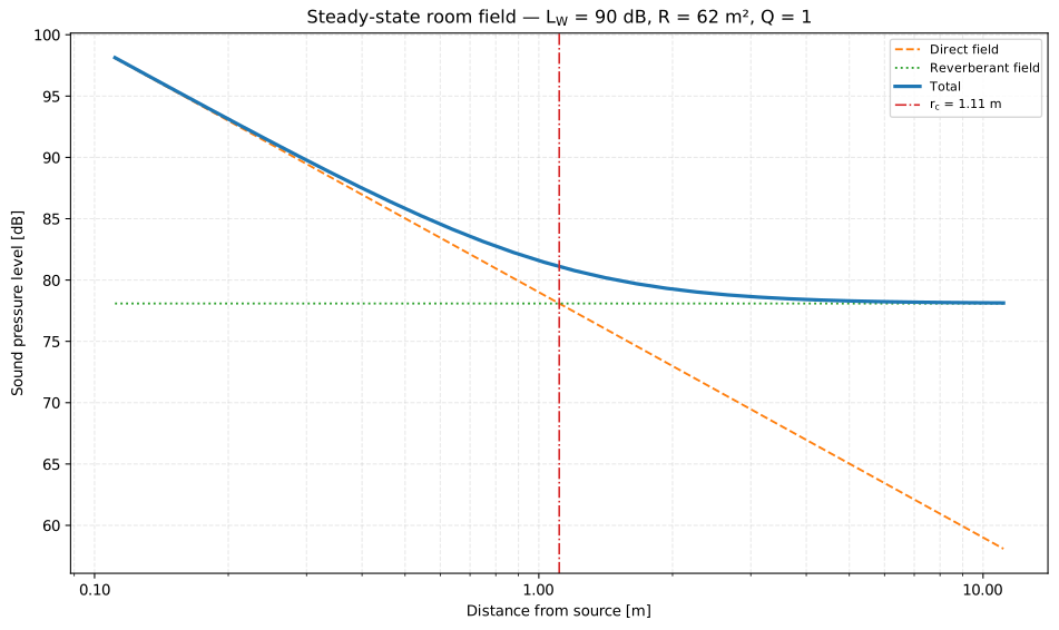
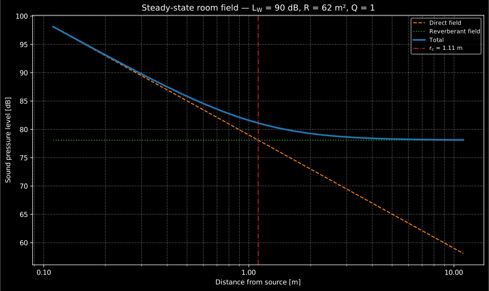
A 90 dB re 1 pW source in a 12 x 8 x 4 m workshop with a mean absorption of 0.15: within $r_{c} = 1.11$ m moving away drops the level 6 dB per doubling; beyond it the reverberant plateau takes over and only absorption, not distance, lowers the level (Bies 5e, §6.4).

Show the code for this figure

import matplotlib.pyplot as plt
import numpy as np
from phonometry import room

field = room.steady_state_field(
    sound_power_level=90.0,     # Lw, dB re 1 pW
    surface_area=352.0,          # a 12 x 8 x 4 m workshop
    mean_absorption=0.15,
)

# One line: direct, reverberant and total levels with rc marked.
field.plot()
plt.show()

# By hand, from the result's fields:
fig, ax = plt.subplots()
ax.semilogx(field.distances, field.direct, "--", label="Direct field")
ax.semilogx(field.distances, field.reverberant, ":", label="Reverberant field")
ax.semilogx(field.distances, field.total, label="Total")
ax.axvline(field.critical_distance, ls="-.",
           label=f"rc = {field.critical_distance:.2f} m")
ax.set_xlabel("Distance from source [m]")
ax.set_ylabel("Sound pressure level [dB]")
ax.legend()
plt.show()

The building blocks are exposed individually, so an emission measurement can flow straight into a level prediction:

from phonometry import room

R = room.room_constant(100.0, 0.2)                     # Bies room constant, 25 m^2
print(round(float(room.critical_distance(R)), 3))      # 0.705 m (Q = 1)
print(round(float(room.steady_state_spl(90.0, 5.0, R)), 2))   # level at 5 m, dB

Kuttruff’s reverberation distance ( $r_{c} = A /16 π$ for $Q = 1$ ) uses the Sabine absorption area $A = S \overset{α}{ˉ}$ rather than the room constant $R = A / (1 - \overset{α}{ˉ})$ ; the two coincide for a small $\overset{α}{ˉ}$ , and this module uses $R$ so that $r_{c}$ is exactly the crossover of its own steady_state_spl. Pass characteristic_impedance=rho_c to add the Bies $10 l g (ρ c /400)$ term (about +0.14 dB at 20 °C).

Where the statistics fade. The Schroeder frequency $f_{s} = 2000 T / V$ (V in m³, T in s) roughly marks the modal-to-diffuse transition, a heuristic crossover rather than a sharp cutoff: well below it discrete modes dominate and the diffuse assumptions of $R$ and $r_{c}$ grow unreliable, well above it the modes overlap and this statistical picture holds. Borderline rooms warrant a band-by-band check.

from phonometry import room
print(round(float(room.schroeder_frequency(1.0, 200.0)), 0))   # 141 Hz

`steady_state_field()` parameters

Parameter	Type	Units	Range / default	Notes
`sound_power_level`	float	dB re 1 pW	—	Source power level `Lw`
`surface_area`	float	m²	> 0	Total boundary area `S`
`mean_absorption`	float	—	`(0, 1)`	Mean Sabine absorption `alpha_bar`
`distances`	1D array, optional	m	> 0	Distance grid (default: `0.1 rc` to `10 rc`)
`directivity`	float	—	> 0, default 1	Source directivity factor `Q`
`characteristic_impedance`	float, optional	Pa·s/m	> 0	Adds the `10 lg(rho c / 400)` term

Returns a SteadyFieldResult (distances, direct, reverberant, total, critical_distance, room_constant) with .plot(). The pieces room_constant, critical_distance, schroeder_frequency and steady_state_spl are also callable directly (each accepting per-band arrays).

Validation

The implementations are checked against the closed forms and the source texts’ own numeric anchors (see the conformance report):

the direct-sound amplitude $1/ (4 π r)$ and delay $r / c$ (exact geometry), the audible image count (Kuttruff 6e, Eq. (9.23)) and the reflection density (Eq. (4.6));
the Eyring reverberation time recovered from the decay of the synthetic RIR in the near-cubic limit (documented ≈ 10 % tolerance), and an independent 2D FDTD solver reproducing the rigid-wall echo delay and the uniform-damping $T_{60}$ ;
the room constant, the critical distance as the exact direct/reverberant crossover, the Schroeder frequency (Kuttruff’s classroom example, $V = 200$ m³, $T = 1$ s → 141 Hz) and the steady-state level (Bies 5e, Eq. (6.43)).

What this guide covers

Covered. Kuttruff’s Room Acoustics (the image-source construction of §4.1, the Eyring reverberation formula used for the near-cubic check and the Schroeder frequency of §3.6), Vorländer’s Auralization (the mirror-source model of Chapter 11, its reflection-factor and delay expressions) and Allen & Berkley’s reflection-order decomposition, all implemented by room.image_source_rir; and the Bies, Hansen & Howard steady-state room field of §6.4 (room constant, directivity $Q$ , critical distance) implemented by room.steady_state_field, room.room_constant, room.critical_distance, room.steady_state_spl and room.schroeder_frequency.

Not covered. The image-source model captures specular reflections only: no diffraction and no diffuse scattering, so an elongated room’s true decay runs slower than the diffuse-field Eyring estimate it is checked against (the anisotropy the Fitzroy and Arau-Puchades models of the reverberation-prediction guide were built to correct). Kuttruff’s alternative reverberation distance (using the Sabine absorption area in place of the room constant) is cited for comparison but not implemented: steady_state_field and critical_distance always use the Bies room-constant formulation.

References

Allen, J. B., & Berkley, D. A. (1979). Image method for efficiently simulating small-room acoustics. The Journal of the Acoustical Society of America, 65(4), 943-950. https://doi.org/10.1121/1.382599The reflection-count decomposition of the rectangular-room image lattice used in §1.
Bies, D. A., Hansen, C. H., & Howard, C. Q. (2017). Engineering noise control (5th ed.). CRC Press. https://doi.org/10.1201/9781351228152The steady-state room field and the room constant of §2 (§6.4).
Kuttruff, H. (2016). Room acoustics (6th ed.). CRC Press. https://doi.org/10.1201/9781315372150The image-source construction (§4.1), the Eyring reverberation and reverberation distance (§5.5–5.6) and the Schroeder frequency (§3.6) of this page.
Vorländer, M. (2020). Auralization: Fundamentals of acoustics, modelling, simulation, algorithms and acoustic virtual reality (2nd ed.). Springer. https://doi.org/10.1007/978-3-030-51202-6The mirror-source model of §1 (Chapter 11), with the reflection-factor and delay expressions.

Created and maintained byJosé Manuel Requena Plens· GitHub· PyPI· All projects