Reverberation-time prediction (Sabine, Eyring, Arau)
Standards: EN 12354ISO 354ISO 9613Key references: Sabine 1922Eyring 1930Millington 1932Fitzroy 1959Arau-Puchades 1988Kuttruff 2016+2 more
The reverberation time , the time for the sound-energy level to fall by 60 dB after the source stops, is predicted here from a room’s volume, boundary areas and the sound-absorption coefficients of its surfaces, through the classical statistical-acoustics formulae. This is the design-stage counterpart of the measured reverberation time of Room acoustics (ISO 3382) and complements the EN 12354-6 model of Sound absorption in enclosed spaces, which specialises the same physics to that standard’s Clause 4.
phonometry offers five models, ordered by how much they account for a non-uniform absorption distribution:
| Model | Absorption term in | Best for |
|---|---|---|
| Sabine | low, uniform absorption | |
| Eyring (Norris-Eyring) | strong, uniform absorption | |
| Millington-Sette | a few very absorptive surfaces | |
| Fitzroy | area-weighted arithmetic mean of three axial Eyring times | anisotropic rooms |
| Arau-Puchades | area-weighted geometric mean of the same three | anisotropic rooms (author-preferred) |
with the Sabine constant (so for ) and the air-absorption term .
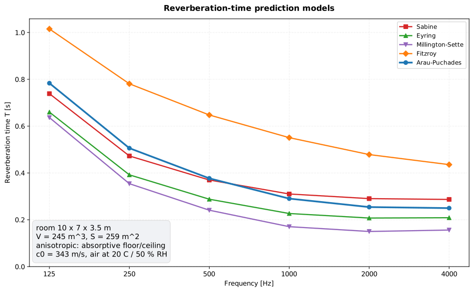
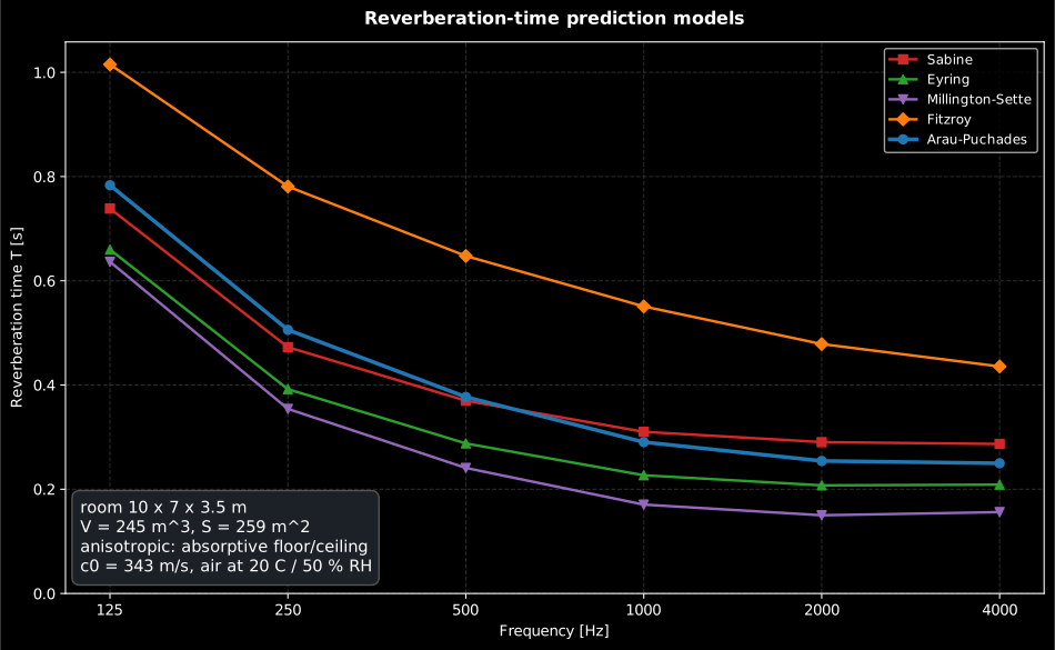
Show the code for this figure
import matplotlib.pyplot as pltfrom phonometry import environmental, room
# A 10 x 7 x 3.5 m room: hard end walls, lightly treated side walls and a# very absorptive floor/ceiling pair (carpet plus an acoustic ceiling).bands = [125.0, 250.0, 500.0, 1000.0, 2000.0, 4000.0]alpha_x = [0.06, 0.07, 0.08, 0.09, 0.10, 0.10]alpha_y = [0.12, 0.14, 0.16, 0.18, 0.20, 0.20]alpha_z = [0.30, 0.50, 0.65, 0.78, 0.82, 0.80]m = environmental.air_attenuation_m(bands, 20.0, 50.0)   # air at 20 C / 50 % RHres = room.reverberation_time_models((10.0, 7.0, 3.5),                                     (alpha_x, alpha_y, alpha_z),                                     air_attenuation=m, frequencies=bands)res.plot()   # the five model curves per bandplt.show()
1. Sabine, Eyring and Millington-Sette
Section titled “1. Sabine, Eyring and Millington-Sette”The three statistical models take the room volume and a list of
(area, absorption_coefficient) surfaces. Sabine is exact only for low,
uniform absorption; Eyring replaces the absorption area by
and is correct where Sabine overestimates ;
Millington-Sette sums the Eyring term surface by surface, so a single
perfectly absorbing surface drives to zero.
from phonometry import room
# A shoebox 8 x 5 x 3 m (V = 120 m3, S = 158 m2), uniform alpha = 0.2.surfaces = [(40.0, 0.2), (40.0, 0.2), (24.0, 0.2),            (24.0, 0.2), (15.0, 0.2), (15.0, 0.2)]print(round(room.sabine_reverberation_time(120.0, surfaces), 3))            # 0.612 sprint(round(room.eyring_reverberation_time(120.0, surfaces), 3))            # 0.548 sprint(round(room.millington_sette_reverberation_time(120.0, surfaces), 3))  # 0.548 s
For a uniform distribution Eyring and Millington-Sette coincide, and both fall below Sabine; Sabine’s over-estimate at high absorption is the reason Eyring exists. As , Eyring reduces to Sabine. Air absorption enters every model through the power-attenuation coefficient (in neper per metre, from the ISO 9613-1 atmospheric absorption):
from phonometry import environmental, room
m = environmental.air_attenuation_m(2000.0, temperature=20.0, relative_humidity=50.0)surfaces = [(40.0, 0.3), (40.0, 0.3), (24.0, 0.3),            (24.0, 0.3), (15.0, 0.3), (15.0, 0.3)]print(round(room.eyring_reverberation_time(120.0, surfaces, air_attenuation=m), 3))
Every statistical model also assumes a diffuse field, and low frequencies break that assumption first: below the Schroeder frequency the room responds as a set of discrete modes, not as a reverberant mixture. The 2D FDTD simulation below drives a rigid 5 m by 3.5 m room exactly on its (2,1) mode and then between two modes; the standing-wave pattern that builds up on resonance is what Sabine and Eyring cannot see.
A 2D FDTD simulation of a rigid 5 by 3.5 metre room driven at the 84 Hz (2,1) mode and at an off-mode frequency side by side. On resonance a standing-wave pattern with fixed nodal lines grows until it dominates the RMS pressure map; off resonance the forced response stays weak and never organises into that nodal structure.
A 2D FDTD simulation of a rigid 5 by 3.5 metre room driven at the 84 Hz (2,1) mode and at an off-mode frequency side by side. On resonance a standing-wave pattern with fixed nodal lines grows until it dominates the RMS pressure map; off resonance the forced response stays weak and never organises into that nodal structure.
2. Fitzroy and Arau-Puchades (anisotropic rooms)
Section titled “2. Fitzroy and Arau-Puchades (anisotropic rooms)”When the absorption is concentrated on one axis (a carpeted floor and an acoustic ceiling against otherwise hard walls), a single mean misrepresents the field. Fitzroy and Arau-Puchades split a rectangular (shoebox) room into the three pairs of opposing walls and combine the axial Eyring reverberation times (each using the whole surface and the mean absorption of the wall pair perpendicular to axis ):
from phonometry import room
# 8 x 5 x 3 m room, absorptive x-wall pair (alpha 0.5), hard elsewhere (0.1).dims = (8.0, 5.0, 3.0)absorption = (0.5, 0.1, 0.1)   # mean alpha of the (x, y, z) wall pairsprint(round(room.arau_puchades_reverberation_time(dims, absorption), 3))  # 0.812 sprint(round(room.fitzroy_reverberation_time(dims, absorption), 3))        # 0.974 s
By the arithmetic-geometric-mean inequality the Arau-Puchades time never exceeds the Fitzroy time; Fitzroy is known to over-predict when one wall pair is very reflective, which is why Arau-Puchades recommends the geometric mean. Both reduce exactly to Eyring for a uniform absorption distribution.
3. Comparing the five models per band
Section titled “3. Comparing the five models per band”reverberation_time_models builds the six boundary surfaces of a rectangular
room from its dimensions and the three wall-pair mean absorptions, then
evaluates all five models on a common footing and returns a
ReverberationModelResult whose .plot() draws the figure above.
from phonometry import room
# 10 x 7 x 3.5 m room, absorptive floor/ceiling against harder walls.res = room.reverberation_time_models(    (10.0, 7.0, 3.5),    (        [0.06, 0.07, 0.08, 0.09, 0.10, 0.10],   # x-pair: hard end walls        [0.12, 0.14, 0.16, 0.18, 0.20, 0.20],   # y-pair: lightly treated walls        [0.30, 0.50, 0.65, 0.78, 0.82, 0.80],   # z-pair: carpet + acoustic ceiling    ),    frequencies=[125.0, 250.0, 500.0, 1000.0, 2000.0, 4000.0],)print(res.sabine.round(2))         # [0.74 0.47 0.37 0.31 0.3  0.3 ]print(res.arau_puchades.round(2))  # [0.79 0.51 0.38 0.29 0.26 0.27]print(res.fitzroy.round(2))        # [1.02 0.79 0.66 0.57 0.51 0.51]res.plot()   # the five model curves per band (the figure above)
Show the code for this figure
import matplotlib.pyplot as pltfrom phonometry import environmental, room
m = environmental.air_attenuation_m([125.0, 250.0, 500.0, 1000.0, 2000.0, 4000.0], 20.0, 50.0)room.reverberation_time_models(    (10.0, 7.0, 3.5),    (        [0.06, 0.07, 0.08, 0.09, 0.10, 0.10],        [0.12, 0.14, 0.16, 0.18, 0.20, 0.20],        [0.30, 0.50, 0.65, 0.78, 0.82, 0.80],    ),    air_attenuation=m,    frequencies=[125.0, 250.0, 500.0, 1000.0, 2000.0, 4000.0],).plot()plt.show()
4. Choosing a model, and when every model fails
Section titled “4. Choosing a model, and when every model fails”The five formulae are not rivals on a single axis of accuracy; each has a domain of validity:
- Sabine is the tool for live rooms with low, reasonably even absorption (mean up to roughly 0.2): classrooms, halls, reverberation chambers. It is also the convention wired into measurement practice, because the ISO 354 absorption coefficient is defined through Sabine’s formula, so feeding reverberation-room data back into Sabine is self-consistent even where the formula is strained. Its structural defect shows at high absorption: with on every surface (an opening in every direction) it still predicts a finite reverberation time.
- Eyring is the choice for evenly treated rooms with substantial absorption: studios, treated offices, listening rooms. It reaches for total absorption, and its correction over Sabine grows with (about 10 % shorter at , 30 % at 0.5).
- Millington-Sette handles a mix of very absorptive and hard surfaces better than a single mean, but it is meant for measured, sub-unity coefficients: a single surface with drives the whole prediction to zero. Reverberation-room coefficients at or above 1.0 (a documented ISO 354 outcome, see the absorption section of Room Acoustics) lie outside the domain of the logarithmic term, so phonometry enforces each formula’s own domain: Sabine accepts such coefficients as supplied (its linear stays finite); Eyring accepts them as long as the mean entering stays below 1 (Fitzroy and Arau-Puchades take the wall-pair means themselves as inputs, so each must already be below 1); Millington-Sette rejects any coefficient at or above 1. To use Millington anyway, bringing such a coefficient into is a modelling decision the formula does not prescribe: whatever adjustment you choose (limiting just below 1 is common), record it alongside the prediction.
- Fitzroy and Arau-Puchades target shoebox rooms whose absorption is concentrated on one axis, the typical office or dwelling with a soft floor and ceiling between hard walls. Arau’s geometric mean tempers Fitzroy’s known over-prediction when one wall pair is very reflective.
When every formula fails. All five inherit the same assumption: a diffuse field, with sound arriving equally from all directions at every point, that stays diffuse while it decays. The common breakages:
- Below the Schroeder frequency the band holds a handful of discrete modes (the animation in §1) and a statistical reverberation time is not defined at all; each mode decays at its own rate set by the wall impedances it actually touches.
- Coupled volumes (a hall with an open stage house, two rooms through a doorway) produce double-slope decays; no single exists, and the measured T20 and T30 disagree (the curvature diagnostic of Room Acoustics).
- Disproportionate rooms (corridors, low flat halls) with the absorption on one surface pair keep a grazing sound field parallel to the hard surfaces that the absorber barely touches; the measured time can be up to twice any statistical prediction, the practical experience recorded in EN 12354-6 (see Sound absorption in enclosed spaces).
- Focusing geometries (domes, curved rear walls) concentrate late energy instead of mixing it, producing position-dependent decays no single-number formula can represent.
Scattering objects restore the mixing the models assume: a furnished room follows the statistical prediction distinctly better than the same room bare, beyond what the furniture’s own absorption area accounts for. In practice, quote a band of predictions (Sabine and Eyring, or Fitzroy and Arau-Puchades for axial cases) rather than a single value; where the models spread, the room is telling you its field is not diffuse.
5. Prediction report (.report())
Section titled “5. Prediction report (.report())”ReverberationModelResult.report(path) renders a one-page PDF fiche of the
prediction: a basis line marking it a design-stage prediction by the five
statistical-acoustics models, an optional metadata header block (client, room,
description, room volume, total surface area, climate), a per-band table with
one reverberation-time column per model beside the model comparison plot
(.plot()), and the boxed mid-frequency reverberation time from Arau-Puchades
(the recommended model for a non-uniform absorption distribution) with the
per-model spread alongside. It is a prediction, not a measurement: the five
models bracket the reverberation time likely to occur, so no PASS/FAIL verdict
is emitted. A target reverberation time supplied through the metadata’s
requirement field is printed as a reference line only, since a room
reverberation time is a target range rather than a strictly
higher/lower-is-better quantity. It uses the same ReportMetadata container and
rendering engine as the other fiches; passing metadata=None produces a bare
prediction fiche. Rendering needs reportlab (pip install phonometry[report]);
only engine="reportlab" is supported. The fiche renders in English by default;
pass language="es" for a Spanish fiche (translated fixed strings and a comma
decimal separator).
from phonometry import reverberation_time_models, ReportMetadata
result = reverberation_time_models(    (8.0, 5.0, 3.0),                       # a shoebox room, one treated wall pair    ([0.10, 0.15, 0.30, 0.45, 0.55, 0.60], # treated wall pair, per octave band     [0.08, 0.10, 0.12, 0.15, 0.18, 0.20], # side walls     [0.05, 0.08, 0.10, 0.12, 0.15, 0.18]),# floor/ceiling    frequencies=[125.0, 250.0, 500.0, 1000.0, 2000.0, 4000.0],)result.report(    "reverberation_fiche.pdf",    metadata=ReportMetadata(        specimen="Classroom, one wall lined with a broadband absorber",        test_room="Classroom C1",        temperature=20.0, relative_humidity=50.0,        laboratory="Phonometry Reference Laboratory",        requirement=0.8,          # printed as a target reference line, no verdict    ),)                                 # the five-model table + the boxed T_mid
The example fiche is regenerated with make reports and kept rendered in the
repository; click the preview to open the PDF.
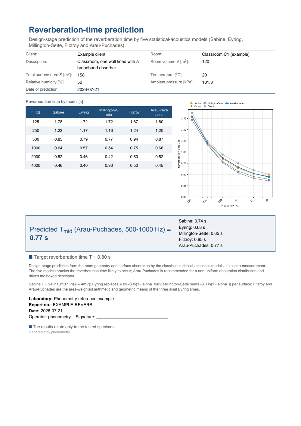
One-page reverberation-time prediction fiche: a metadata header (client, room, description, room volume, total surface area, temperature, humidity and pressure), the octave-band table with one reverberation-time column per model (Sabine, Eyring, Millington-Sette, Fitzroy and Arau-Puchades from 125 Hz to 4 kHz) beside the five-model comparison plot, the boxed mid-frequency reverberation time from Arau-Puchades with the per-model spread alongside, and a target reverberation-time reference line (no PASS/FAIL verdict).
What this guide covers
Section titled “What this guide covers”Covered. The classical statistical-acoustics reverberation-time formulae
of Sabine (1922), Eyring (1930), Millington-Sette (1932), Fitzroy (1959) and
Arau-Puchades (1988), each with its own domain-of-validity check and the
ISO 9613-1-derived air-absorption term, via room.sabine_reverberation_time,
room.eyring_reverberation_time, room.millington_sette_reverberation_time,
room.fitzroy_reverberation_time, room.arau_puchades_reverberation_time
and the combined room.reverberation_time_models.
Not covered. EN 12354-6’s own Clause 4 model (a Sabine calculation with an added object term and the ISO 9613-1 air term) is a distinct, standard-defined calculation that lives in the Sound absorption in enclosed spaces guide, not here. None of the five formulae here models coupled volumes, disproportionate rooms or focusing geometries: their double-slope or position-dependent decays fall outside every diffuse-field assumption (§4). For a measured decay that shows those symptoms, use the T20/T30 curvature diagnostic of the Room Acoustics guide rather than a statistical prediction.
See also
Section titled “See also”- API reference:
room.reverberation_predictionandenvironmental.air_absorption.
References
Section titled “References”- Arau-Puchades, H. (1988). An improved reverberation formula. Acustica, 65(4), 163-180. The geometric-mean combination of §2 (its Formula 18). The linked record is the publisher page at Ingenta.
- Carrión Isbert, A. (1998). Diseño acústico de espacios arquitectónicos. Edicions UPC. A Spanish-language textbook treatment of the reverberation models and their use in room design. ISBN 978-84-8301-252-9.
- European Committee for Standardization. (2003). Building acoustics — Estimation of acoustic performance of buildings from the performance of elements — Part 6: Sound absorption in enclosed spaces (EN 12354-6:2003). The classical formulae predate the normative world and enter it through this standard, whose Clause 4 model is a Sabine calculation with object and air terms; see the enclosed-space absorption guide. The linked catalogue record is the BSI Knowledge page for BS EN 12354-6:2003.
- Everest, F. A. (2001). Master handbook of acoustics (4th ed.). McGraw-Hill. The Fig. 7-22 worked example the conformance suite reproduces: Example 1, an untreated 23.3 × 16 × 10 ft room, whose six printed Sabine reverberation times the SI implementation reproduces to ≤ 0.02 s, reinforced by hand-computed closed-form values and the model identities (every model collapses to Eyring for uniform absorption; Eyring collapses to Sabine as the absorption tends to zero), which transitively carry that real-data anchor to the whole family. ISBN 978-0-07-136097-5.
- Eyring, C. F. (1930). Reverberation time in "dead" rooms. The Journal of the Acoustical Society of America, 1(2A), 217-241. https://doi.org/10.1121/1.1915175The mean-free-path derivation behind the −S ln(1−ᾱ) term of §1.
- Fitzroy, D. (1959). Reverberation formula which seems to be more accurate with nonuniform distribution of absorption. The Journal of the Acoustical Society of America, 31(7), 893-897. https://doi.org/10.1121/1.1907814The axial split into three wall-pair decays of §2.
- International Organization for Standardization. (1993). Acoustics — Attenuation of sound during propagation outdoors — Part 1: Calculation of the absorption of sound by the atmosphere (ISO 9613-1:1993). The atmospheric-absorption coefficient behind the air term 4mV; see the outdoor propagation guide.
- International Organization for Standardization. (2003). Acoustics — Measurement of sound absorption in a reverberation room (ISO 354:2003). Defines the measured absorption coefficient via Sabine's formula, the self-consistency argument of §4.
- Kuttruff, H. (2016). Room acoustics (6th ed.). CRC Press. https://doi.org/10.1201/9781315372150The diffuse-field theory, its limits and the modern assessment of the classical formulae behind §4.
- Millington, G. (1932). A modified formula for reverberation. The Journal of the Acoustical Society of America, 4(1), 69-82. https://doi.org/10.1121/1.1915588The per-surface logarithmic absorption term of §1.
- Sabine, W. C. (1922). Collected papers on acoustics. Harvard University Press. The original reverberation experiments and the T = 0.161 V/A law of §1. The linked copy is the free scan at the Internet Archive.