Correlation, time delay and envelope

Where the calibrated spectral estimators describe a signal in frequency, this page covers their time-domain counterparts in phonometry.metrology: auto- and cross-correlation estimates with the three standard normalizations and their Bendat & Piersol random errors; time-delay estimation (TDE) by the direct correlator, the cross-spectrum phase slope and the generalized cross-correlation (GCC) of Knapp & Carter with the Roth, SCOT, PHAT and maximum-likelihood weightings; sub-sample peak location for impulse-response delays and alignment; and the Hilbert envelope with instantaneous phase and frequency. The GCC estimators run on the same Welch core as the spectral densities, so both views of a signal pair are mutually consistent bin by bin.

1. Correlation estimates

correlation computes the auto- or cross-correlation via zero-padded FFT so the circular product never wraps (Bendat & Piersol Section 11.4.2), with the sign convention of the book’s time-delay model: for y(t) = α·x(t-τ0) + n(t) the estimate peaks at τ = +τ0 (Eq. 5.21). Three normalizations are available:

• 'biased': the lag sums divided by N; tapers toward the record ends and stays bounded by [Rxx(0)·Ryy(0)]^1/2;
• 'unbiased': divided by N-|r| (Eq. 11.96), an unbiased estimate of Rxy(τ) whose variance grows toward the ends;
• 'coefficient': the correlation coefficient function ρxy(τ) = Cxy(τ)/(σx·σy) in [-1, 1] over the mean-removed records (Eq. 5.16).

import numpy as np
from phonometry import correlation

res = correlation(x, y, fs, normalization="coefficient", max_lag=0.05)
peak = np.argmax(res.values)
print(res.lags[peak], res.values[peak])   # delay and its coefficient
res.plot()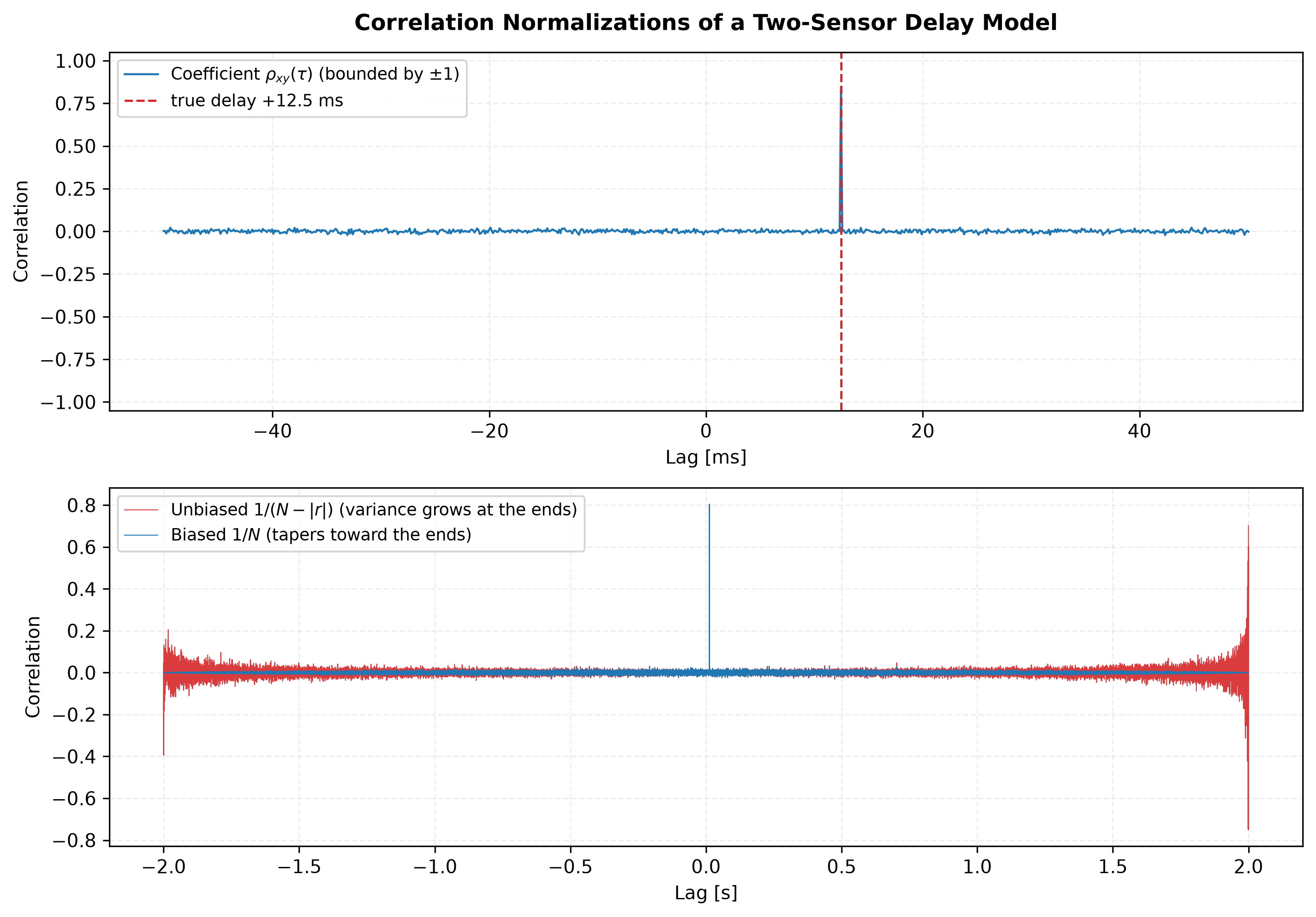

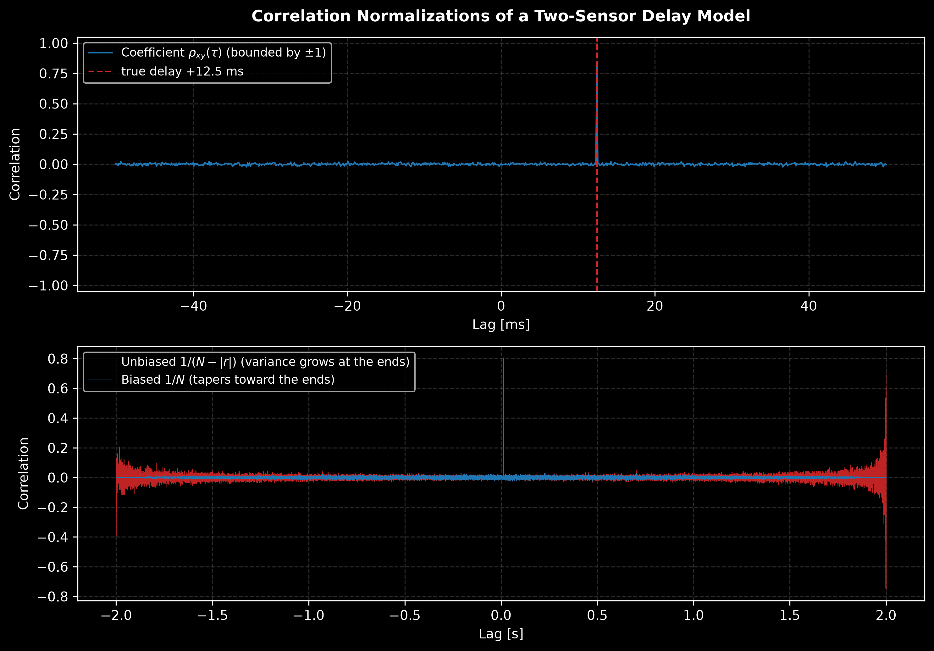
The two-sensor delay model y(t) = 0.8·x(t−τ0) + n(t) under the three normalizations: the coefficient function is bounded and peaks at +τ0 (top); over the full lag range the biased estimate tapers toward the ends while the unbiased one pays for its unbiasedness with variance that grows there (bottom).

Show the code for this figure

import matplotlib.pyplot as plt
import numpy as np
from phonometry import correlation, noise_signal

fs = 8192.0
delay = 102                                  # 12.45 ms
x = noise_signal(fs, 2.0, seed=4)
interference = noise_signal(fs, 2.0, rms=0.5, seed=5)
y = 0.8 * np.concatenate([np.zeros(delay), x[:-delay]]) + interference

res = correlation(x, y, fs, normalization="coefficient", max_lag=0.05)

# One line — the correlation estimate against the lag in seconds:
res.plot()
plt.show()

# The three normalizations by hand, from the same records:
biased = correlation(x, y, fs, normalization="biased")
unbiased = correlation(x, y, fs, normalization="unbiased")

fig, (ax_c, ax_n) = plt.subplots(2, 1)
ax_c.plot(1e3 * res.lags, res.values, label="coefficient")
ax_c.axvline(1e3 * delay / fs, color="r", linestyle="--",
             label="true delay")
ax_c.set(xlabel="Lag [ms]", ylabel="Correlation")
ax_n.plot(unbiased.lags, unbiased.values, "r", lw=0.5, label="unbiased")
ax_n.plot(biased.lags, biased.values, lw=0.5, label="biased")
ax_n.set(xlabel="Lag [s]", ylabel="Correlation")
for ax in (ax_c, ax_n):
    ax.legend()
plt.show()

The result always carries the coefficient function alongside the requested normalization, because the coefficient is what the error formulas need. For bandwidth-limited Gaussian data of bandwidth B observed for T seconds (Eqs. 8.109/8.112, valid for T ≥ 10·|τ| and BT ≥ 5):

$$\epsilon \left[{\hat{R}}_{xy}(\tau )\right]=\frac{{\left[1+{\rho }_{xy}^{-2}(\tau )\right]}^{1/2}}{\sqrt{2BT}},\epsilon \left[{\hat{R}}_{xx}(0)\right]=\frac{1}{\sqrt{BT}}.$$

res.random_error(signal_bandwidth) evaluates it per lag with the measured coefficient, and the standalone correlation_random_error takes an explicit coefficient; with ρ = S/√((S+M)(S+N)) = 1/11, B = 100 Hz and T = 5 s it reproduces the ε ≈ 0.35 of the book’s Example 8.5, one of the pinned conformance anchors. Two closed forms anchor the estimator itself in the tests: the autocorrelation of a sine, (A²/2)·cos(2πf0τ), and the sin(2πBτ)/(2πBτ) autocorrelation of bandwidth-limited white noise (Eq. 8.120).

2. Time-delay estimation

time_delay estimates the delay of y relative to x in the two-sensor model y(t) = α·x(t-τ0) + n(t) (B&P Section 5.1.4) by three routes:

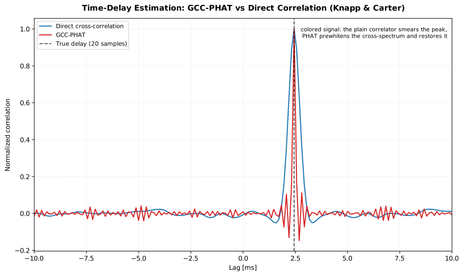
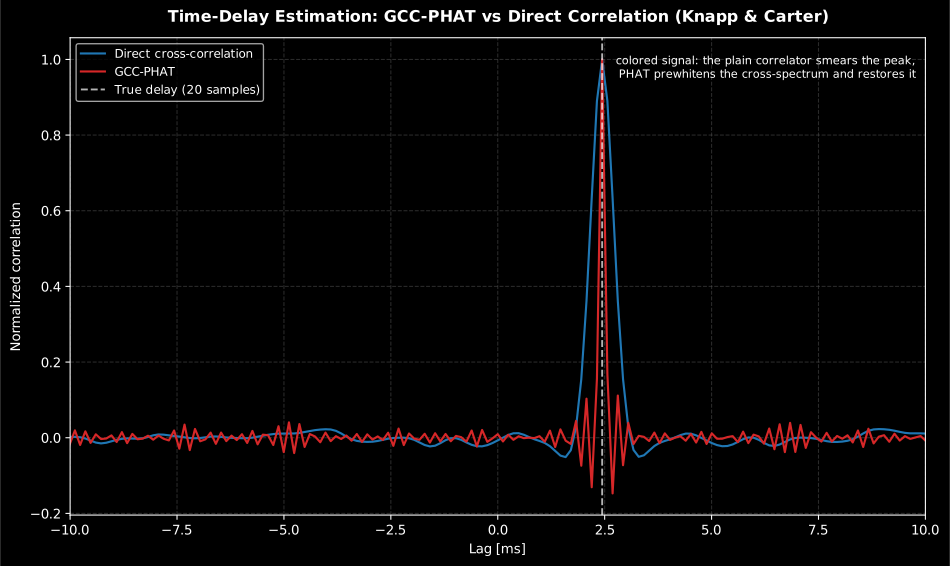
• 'direct': the peak of the full-record correlation coefficient function;
• 'phase': the |Gxy|-weighted least-squares slope of the cross-spectrum phase (Eq. 5.101b): a pure delay has an exactly linear phase, so this estimator resolves fractional delays to better than 1e-3 samples without any peak interpolation, as long as the unwrapped phase is unambiguous (clean, moderate delays);
• 'gcc': the generalized cross-correlation of Knapp & Carter (1976): the Welch-averaged cross-spectrum is weighted by ψ(f) before the inverse transform, sharpening the peak that the signal’s own autocorrelation would otherwise smear (their Eq. 9).

The weightings of Knapp & Carter’s Table I, with the conditions the paper attaches to each:

weighting	ψ(f)	Behaviour and conditions
'none'	1	The plain correlator: the delta at the delay is convolved with the signal autocorrelation, giving a broad peak on colored signals.
'roth'	1/Gxx	Suppresses the bands where the first sensor is noisy; still smears unless that noise is spectrally similar to the signal.
'scot'	1/√(Gxx·Gyy)	Prewhitens both channels symmetrically; equals Roth when the sensors match.
'phat'	`1/	Gxy
'ml'	`γ²/(	Gxy

Show the code for this figure

import matplotlib.pyplot as plt
import numpy as np
from scipy import signal as sp_signal
from phonometry import noise_signal, time_delay

fs = 8192.0
delay = 20  # samples
b, a = sp_signal.butter(2, 800.0 / (fs / 2.0))   # colored common signal
s = sp_signal.lfilter(b, a, noise_signal(fs, 4.0, color="white", seed=10))
x = s + noise_signal(fs, 4.0, color="white", rms=0.02, seed=11)
y = np.roll(s, delay) + noise_signal(fs, 4.0, color="white", rms=0.02, seed=12)

direct = time_delay(x, y, fs, method="direct", max_delay=0.01)
phat = time_delay(x, y, fs, method="gcc", weighting="phat",
                  nperseg=2048, max_delay=0.01)

fig, ax = plt.subplots(figsize=(10, 6))
ax.plot(1e3 * direct.lags,
        direct.correlation / np.max(np.abs(direct.correlation)),
        label="Direct cross-correlation")
ax.plot(1e3 * phat.lags, phat.correlation, label="GCC-PHAT")
ax.axvline(1e3 * delay / fs, ls="--", color="k", label="True delay")
ax.set_xlabel("Lag [ms]")
ax.set_ylabel("Normalized correlation")
ax.legend()
plt.show()

The correlation-peak methods refine the sample peak by three-point parabolic interpolation, optionally after band-limited local upsampling (upsample=16 resamples a window around the peak sixteenfold before the parabola). Sub-sample accuracy presumes the peak is oversampled, i.e. the signals are band-limited below Nyquist; on a 0.4·fs band-limited pair the tests pin the achievable error at ≲0.1 sample for the parabola alone and ≲2e-3 samples with upsample=16. For GCC the delay must fit within half a Welch segment; raise nperseg for longer delays.

With signal_bandwidth given, the result also carries the peak-location uncertainty of B&P Eq. 8.129 and its ±2σ interval (Eq. 8.130):

$$\sigma ({\hat{\tau }}_0)\approx {\left(\frac{3}{4}\right)}^{1/4}\frac{\sqrt{\epsilon [{\hat{R}}_{xy}({\tau }_0)]}}{\pi B}.$$

from phonometry import time_delay

res = time_delay(x, y, fs, method="gcc", weighting="ml",
                 nperseg=2048, upsample=16, signal_bandwidth=1000.0)
print(res.delay, res.delay_samples)     # seconds and fractional samples
print(res.delay_std, res.delay_interval)  # Eq. 8.129 sigma, +/-2 sigma
res.plot()                              # correlation with the delay marked

The formula models the peak of the continuous correlation function, so treat the interval as a conservative order-of-magnitude bound; the seeded Monte Carlo in the test suite observes the actual scatter below the prediction.

3. Impulse-response delay and alignment

The cross-correlation of an impulse response with an ideal unit impulse is the IR itself, so the sub-sample location of its peak magnitude is its arrival time. impulse_response_delay applies exactly the same refinement as the TDE peak (local band-limited upsampling, default ×8, plus the parabola), and with a reference IR it measures the delay between the pair from their full-record cross-correlation (one-shot transients are not stationary records, so the direct correlator is used rather than the Welch-averaged GCC):

from phonometry import align_impulse_responses, impulse_response_delay

t_arrival = impulse_response_delay(ir, fs)              # seconds from t = 0
dt = impulse_response_delay(ir_b, fs, reference=ir_a)   # pair delay

res = align_impulse_responses(ir_b, ir_a, fs)  # remove the estimated delay
res.plot()                                     # reference vs aligned overlay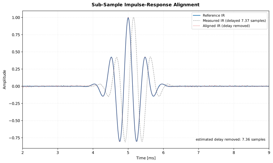

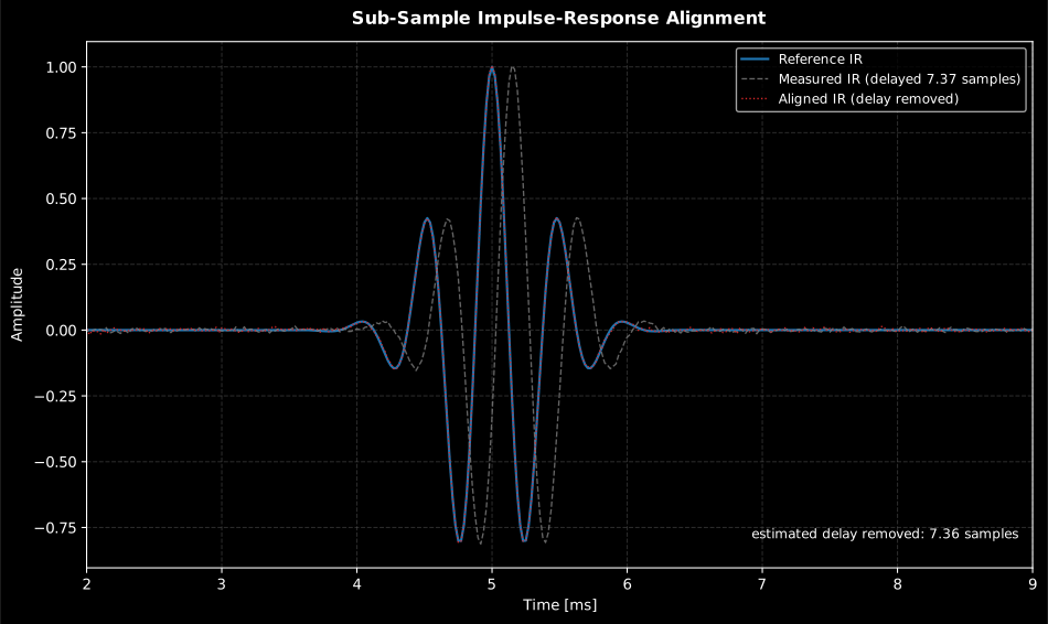
A measured IR delayed by a fractional 7.37 samples (dashed) is aligned back onto its reference: the band-limited shift removes the estimated 7.36 samples and the aligned trace (dotted) lands on the reference.

Show the code for this figure

import matplotlib.pyplot as plt
import numpy as np
from scipy import signal as sp_signal
from phonometry import align_impulse_responses, fractional_delay

fs = 48000.0
t = np.arange(int(0.03 * fs)) / fs
rng = np.random.default_rng(6)
# Band-limited reference pulse: a 2 kHz Gaussian tone burst at 5 ms.
ir_a = sp_signal.gausspulse(t - 0.005, fc=2000.0, bw=0.5)
ir_b = fractional_delay(ir_a, 7.37)[: ir_a.size]
ir_b += 0.005 * rng.standard_normal(ir_a.size)

res = align_impulse_responses(ir_b, ir_a, fs)

# One line — reference and aligned IR overlaid:
res.plot()
plt.show()

# By hand, from the fields the result carries:
t_ms = 1e3 * t
fig, ax = plt.subplots()
ax.plot(t_ms, res.reference, lw=1.6, label="Reference IR")
ax.plot(t_ms, ir_b, "0.5", lw=1.0, linestyle="--", label="Measured IR")
ax.plot(t_ms, res.aligned[: t.size], "r:", label="Aligned IR")
ax.set(xlabel="Time [ms]", ylabel="Amplitude",
       title=f"delay removed: {res.delay_samples:.2f} samples")
ax.legend()
plt.show()

align_impulse_responses removes the estimated delay with an exact band-limited fractional shift (a frequency-domain phase ramp over a zero-padded record, so nothing wraps around): the tool for averaging IR ensembles or comparing measurements taken at slightly different distances. The synthetic fractional-delay tests document the achievable accuracy on a smooth band-limited pulse: about 1e-2 samples with the parabola alone, 1e-3 at the default upsample=8, below 1e-5 at ×32.

4. Hilbert envelope and instantaneous frequency

envelope builds the analytic signal z(t) = x(t) + j·x̃(t) by the one-sided spectrum construction that Bendat & Piersol recommend (Eq. 13.25) and returns the three Chapter 13 quantities on one time axis:

$$A(t)={\left[x^2(t)+{\tilde{x}}^2(t)\right]}^{1/2},\theta (t)=\arctan \frac{\tilde{x}(t)}{x(t)},f(t)=\frac{1}{2\pi }\frac{d\theta }{dt}.$$

For an amplitude-modulated carrier u(t)·cos(2πf0t) the envelope recovers u(t) exactly (Eq. 13.27); the conformance suite pins the recovered AM envelope and the Table 13.1 pair cos → sin at the 1e-9 level, and the instantaneous frequency of a chirp tracks its sweep.

from phonometry import envelope

res = envelope(x, fs)
print(res.envelope, res.instantaneous_frequency)
res.plot()               # signal + envelope, instantaneous frequency

slow = envelope(x, fs, decimation_factor=32)   # anti-aliased, fs/32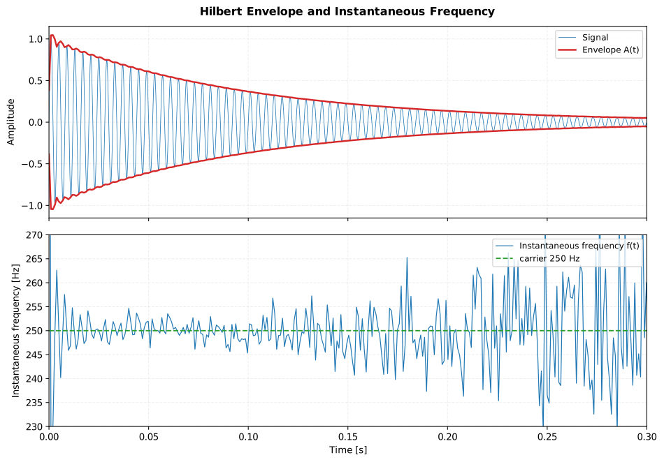

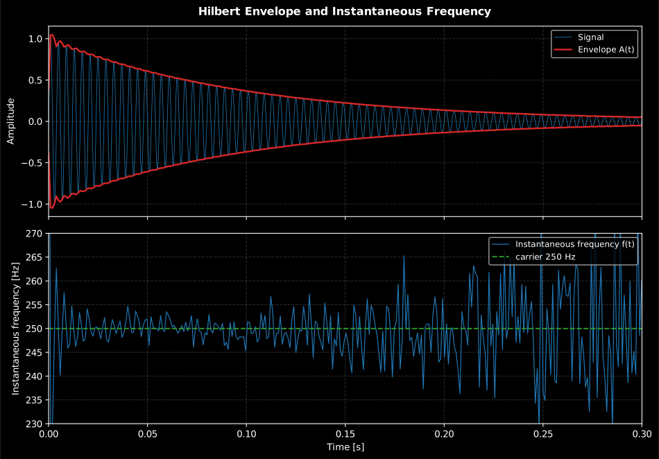
The Hilbert quantities of a struck 250 Hz mode: the envelope traces the exponential decay (top), and the instantaneous frequency sits on the carrier while the mode dominates, jittering as the signal sinks into the noise floor (bottom, ×8 anti-aliased decimation).

Show the code for this figure

import matplotlib.pyplot as plt
import numpy as np
from phonometry import envelope

fs = 8192.0
t = np.arange(int(0.4 * fs)) / fs
rng = np.random.default_rng(7)
x = np.exp(-t / 0.1) * np.sin(2 * np.pi * 250.0 * t)   # a struck mode
x += 0.001 * rng.standard_normal(t.size)

res = envelope(x, fs, decimation_factor=8)

# One line — signal + envelope and the instantaneous frequency:
res.plot()
plt.show()

# By hand, from the fields the result carries:
fig, (ax_e, ax_f) = plt.subplots(2, 1, sharex=True)
ax_e.plot(t, res.signal, lw=0.6, label="Signal")
ax_e.plot(res.times, res.envelope, "r", lw=1.8, label="Envelope A(t)")
ax_e.plot(res.times, -res.envelope, "r", lw=1.8)
ax_e.legend()
ax_f.plot(res.times, res.instantaneous_frequency, lw=0.9,
          label="Instantaneous frequency f(t)")
ax_f.axhline(250.0, color="g", linestyle="--", label="carrier 250 Hz")
ax_f.set(xlabel="Time [s]", ylabel="Frequency [Hz]", ylim=(230, 270))
ax_f.legend()
plt.show()

The envelope of a band-limited signal is itself low-frequency, so the result offers optional decimation: a zero-phase FIR anti-alias filter by default, or plain subsampling with antialias=False, exactly the convention the ECMA-418-2 loudness/roughness chain of phonometry.psychoacoustics applies internally after its auditory bandpass (Formulae 65/119 of the standard), appropriate when the input is already narrowband.

Relation to the spectral estimators

time_delay (GCC and phase methods) runs on the same Welch core (taper, overlap policy, detrend-off calibration, segment defaults) as cross_spectral_density and the H1/H2 frequency-response estimators, so a GCC, a coherence and a cross-spectrum computed with the same segment length agree bin by bin; the 'phase' estimator is literally the slope of the CrossSpectralDensityResult phase, weighted as Eq. 5.101b prescribes.

The Hilbert envelope here is the time-domain companion of the envelope spectrum, which reads the same modulations off as discrete lines in frequency; and the sub-sample alignment shares its band-limited kernel with the public fractional-delay and resampling tools.

What this guide covers

Covered. Bendat & Piersol Chapter 5, Section 8.4 and Chapter 13: correlation with the biased, unbiased and coefficient normalizations and their random-error formulas (Eqs. 8.109/8.112); time_delay with the direct, phase-slope and Knapp & Carter (1976) generalized cross-correlation methods, including the Roth, SCOT, PHAT and maximum-likelihood weightings of their Table I; the peak-location uncertainty of Eq. 8.129; impulse_response_delay and align_impulse_responses; and the Hilbert envelope with instantaneous phase and frequency (Chapter 13).

Not covered. correlation and time_delay model a single common-path delay between exactly two sensors (the y(t) = α·x(t-τ0) + n(t) model of Eq. 5.21). A record with several arrivals (multipath, a direct path plus reflections) is not separated automatically: time_delay and the direct correlator report only the single largest peak, the same limitation echo_detection names on the cepstrum in Cepstrum, echoes and the envelope spectrum. Estimating delays across more than two sensors, as an array or beamformer would, means calling these pairwise functions yourself; there is no built-in multi-sensor TDOA solver.

References

• Bendat, J. S., & Piersol, A. G. (2010). Random data: Analysis and measurement procedures (4th ed.). Wiley. https://doi.org/10.1002/9781118032428Sections 5.1.4 and 5.2.6-5.2.7 (time delay via correlation and cross-spectrum), 8.4 (random errors of correlation estimates and of the peak location), 11.4 (FFT computation with zero padding) and Chapter 13 (Hilbert transforms, envelope and instantaneous phase). ISBN 978-0-470-24877-5.
• Knapp, C. H., & Carter, G. C. (1976). The generalized correlation method for estimation of time delay. IEEE Transactions on Acoustics, Speech, and Signal Processing, 24(4), 320-327. https://doi.org/10.1109/TASSP.1976.1162830The GCC framework, the Table I weightings and their conditions, and the maximum-likelihood (Hannan-Thomson) processor.