Multiple and partial coherence

When several partially correlated sources drive one response, the ordinary coherence of each source with the output is misleading. A source that only correlates with the true cause inherits a spurious coherence through it, so reading the ordinary coherences alone can credit the wrong source. Bendat & Piersol, Random Data (4th ed., 2010, Chapter 7), resolve this for a multiple-input/single-output (MISO) system with the multiple and partial coherence functions. miso_coherence computes them from the same Welch cross-spectral core as the rest of phonometry.metrology, for several correlated inputs and one output.

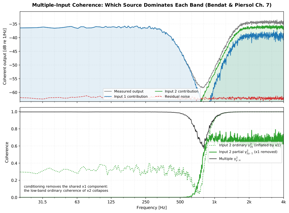
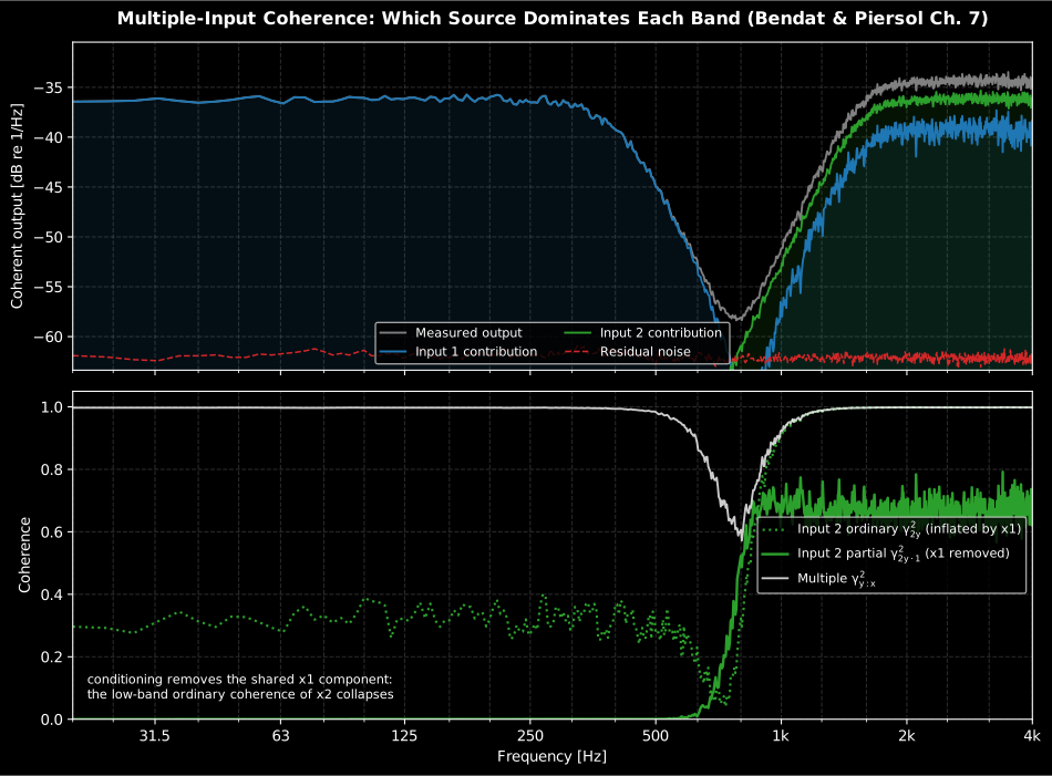
Show the code for this figure

import matplotlib.pyplot as plt
import numpy as np
from scipy import signal
from phonometry import miso_coherence, noise_signal

fs = 8192.0
# Input 1 drives a low-frequency path; input 2 = 0.7*x1 + independent noise
# drives a high-frequency path, so input 2 is correlated with input 1.
x1 = noise_signal(fs, 32.0, color="white", seed=1)
x2 = 0.7 * x1 + noise_signal(fs, 32.0, color="white", seed=2)
low = signal.butter(4, 400.0, fs=fs, output="sos")
high = signal.butter(4, 1500.0, btype="high", fs=fs, output="sos")
noise = noise_signal(fs, 32.0, color="white", rms=0.05, seed=3)
y = signal.sosfilt(low, x1) + signal.sosfilt(high, x2) + noise

res = miso_coherence([x1, x2], y, fs, nperseg=2048)
f = res.frequencies
band = (f >= 20.0) & (f <= 4000.0)

fig, (ax_top, ax_bot) = plt.subplots(2, 1, figsize=(10, 7.4), sharex=True)
db = lambda v: 10 * np.log10(v)
ax_top.semilogx(f[band], db(res.output_psd[band]), color="gray",
                label="Measured output")
for i, color in ((0, "#1f77b4"), (1, "#2ca02c")):
    ax_top.semilogx(f[band], db(res.coherent_output_spectra[i][band]),
                    color=color, label=f"Input {i + 1} contribution")
ax_top.semilogx(f[band], db(res.noise_psd[band]), "--", color="#d62728",
                label="Residual noise")
ax_top.set_ylabel("Coherent output [dB re 1/Hz]")
ax_top.legend()

ax_bot.semilogx(f[band], res.ordinary_coherence[1][band], ":", color="#2ca02c",
                label="Input 2 ordinary (inflated by x1)")
ax_bot.semilogx(f[band], res.partial_coherence[1][band], color="#2ca02c",
                label="Input 2 partial (x1 removed)")
ax_bot.semilogx(f[band], res.multiple_coherence[band], color="black",
                label="Multiple")
ax_bot.set_xlabel("Frequency [Hz]")
ax_bot.set_ylabel("Coherence")
ax_bot.set_ylim(0, 1.05)
ax_bot.legend()
plt.show()

The .plot() method draws the same two panels in one call:

res.plot()          # English labels; res.plot(language="es") for Spanish

1. Ordinary, multiple and partial coherence

For a system with q inputs x1..xq and output y, miso_coherence estimates every auto- and cross-spectrum by Welch’s method and reports three coherence functions.

The ordinary coherence of input i with the output, on its own (Eq. 7.109), is the familiar single-input quantity:

$${\gamma }_{iy}^2(f)=\frac{|G_{iy}(f){|}^2}{G_{ii}(f)G_{yy}(f)}.$$

The multiple coherence (Eq. 7.35) is the fraction of the output autospectrum linearly explained by all inputs jointly. From the Hermitian input cross-spectral matrix Gxx and the input-output vector Gxy it is

$${\gamma }_{y:x}^2(f)=\frac{G_{xy}^H{G}_{xx}^{-1}{G}_{xy}}{G_{yy}}=1-\frac{G_{nn}}{G_{yy}},$$

where Gnn is the residual output spectrum uncorrelated with every input. If the output carries additive uncorrelated noise of per-band signal-to-noise ratio SNR, this is exactly $\mathrm{SNR}/(1+\mathrm{SNR})$, the closed-form oracle used to verify the implementation.

The partial coherence of input i (Eq. 7.87) is its coherence with the output once the linear effect of the inputs before it in the conditioning order has been removed:

$${\gamma }_{iy\cdot (i-1)!}^2(f)=\frac{|G_{iy\cdot (i-1)!}(f){|}^2}{G_{ii\cdot (i-1)!}(f)G_{yy}(f)}.$$

The 4th-edition definition keeps the total output Gyy in the denominator (not the conditioned output). That choice makes the partial coherences of the ordered inputs sum to the multiple coherence, ${\gamma }_{y:x}^2={\sum }_i{\gamma }_{iy\cdot (i-1)!}^2$ (Eq. 7.116), and reduce exactly to the ordinary coherences when the inputs are mutually uncorrelated (Eq. 7.117).

res = miso_coherence([x1, x2], y, fs)
res.ordinary_coherence   # shape (q, F): each input on its own
res.multiple_coherence   # shape (F,):  all inputs jointly
res.partial_coherence    # shape (q, F): conditioned on the preceding inputs

2. Conditioning: separating cause from correlation

The partial coherences come from the conditioned spectra Gij·r!, computed by the Gaussian-elimination recursion of Section 7.3. Removing the linear effect of a pivot input r from every remaining record is one Schur complement step (Eq. 7.94):

$$G_{ij\cdot r!}=G_{ij\cdot (r-1)!}-\frac{G_{rj\cdot (r-1)!}{G}_{ir\cdot (r-1)!}}{G_{rr\cdot (r-1)!}},$$

applied for each input in the conditioning order until only the residual output spectrum Gyy·q! remains. This is the whole point of the method: in the figure above, input 2 is 0.7·x1 + independent noise, so it correlates with input 1 but drives no low-frequency path. Its ordinary coherence with the output therefore reads about 0.3 across the low band, borrowed entirely through input 1, while its partial coherence collapses to zero there once input 1 is conditioned out.

low = (res.frequencies > 100.0) & (res.frequencies < 300.0)
res.ordinary_coherence[1][low].mean()   # ~0.32  (inflated through x1)
res.partial_coherence[1][low].mean()    # ~0.00  (x1 removed)

3. Which source dominates each band

The conditioning also splits the output power source by source. The partial coherent output spectrum of input i (Eq. 7.86) is the share of the output autospectrum it contributes, and the shares plus the residual noise reconstruct the output exactly (Eqs. 7.88/7.121):

$$G_{v_i}={\gamma }_{iy\cdot (i-1)!}^2{G}_{yy},\sum _i{G}_{v_i}+G_{nn}=G_{yy}.$$

Comparing the shares band by band answers “which source dominates here?”. dominant_input() returns, for every frequency, the index of the input with the largest share:

res.coherent_output_spectra        # shape (q, F): Gvi per input
dominant = res.dominant_input()    # index of the strongest source per bin
f = res.frequencies
dominant[np.argmin(abs(f - 200.0))]    # 0 (input 1 drives the low band)
dominant[np.argmin(abs(f - 2500.0))]   # 1 (input 2 drives the high band)

4. Statistical quality and the conditioning order

The random errors follow Section 9.3. Conditioning on the i-1 preceding inputs costs i-1 degrees of freedom, so the i-th ordered input carries nd-(i-1) effective averages (Eqs. 9.100/9.101) and the q-input multiple coherence carries nd-(q-1) (Eq. 9.98). The result exposes multiple_coherence_random_error and coherent_output_random_error alongside the effective average count n_averages.

The ordinary and multiple coherences do not depend on the conditioning order, but the partial coherences and the coherent-output decomposition do: each input is conditioned on whatever precedes it. Absent a physical ordering, Bendat & Piersol (Section 7.2.4) recommend ordering the inputs by descending ordinary coherence with the output. Pass order to choose:

res = miso_coherence([x1, x2, x3], y, fs, order=(2, 0, 1))
res.order            # (2, 0, 1): the order actually applied
res.plot()           # the two panels, recomputed in the applied order

Two practical pitfalls are worth naming. Averaging: every conditioning step spends a degree of freedom, so with few segments the partial coherences of the last-ordered inputs are the least trustworthy numbers on the page; average generously before reading a small partial coherence as zero. Delay bias: like the ordinary coherence, the Welch estimate is biased low when a bulk delay between an input and the output becomes a noticeable fraction of the segment length; remove known propagation delays first (see Correlation and delay) and keep nperseg well above the longest remaining delay.

The estimators share the Welch core of the calibrated spectral analysis page (same Hann taper, 50 % overlap and detrend-off calibration), so a MISO coherence and a power_spectral_density computed with the same segment length are consistent bin by bin.

What this guide covers

Covered. Bendat & Piersol Chapter 7’s ordinary, multiple and partial coherence functions (Eqs. 7.109, 7.35, 7.87), the Gaussian-elimination conditioning recursion (Eq. 7.94), the partial coherent output spectra and their exact decomposition of the output (Eqs. 7.86/7.116/7.121), and the Section 9.3 random errors of the multiple and conditioned estimates (Eqs. 9.98-9.101), all exposed by miso_coherence and MISOCoherenceResult.

Not covered. The chapter’s multiple-input frequency-response (gain factor Liy) estimates, the linear model that predicts the output from the conditioned inputs, are computed internally to build the coherent output spectra but are not returned: MISOCoherenceResult exposes the coherence and spectral-decomposition side only, not a fitted multi-input transfer function. The method is also single-output (MISO); a system with several correlated outputs needs one miso_coherence call per output.

See also

• Spectral analysis: the single-input coherent output spectrum this page generalizes, and the shared Welch core.
• Correlation and delay: estimating and removing the bulk delays that bias coherence low.
• Multichannel and Performance: the per-channel path this cross-channel analysis complements.
• API reference: metrology.miso.

References

• Bendat, J. S., & Piersol, A. G. (2010). Random data: Analysis and measurement procedures (4th ed.). Wiley. https://doi.org/10.1002/9781118032428Chapter 7 (multiple-input/output relationships: ordinary coherence Eq. 7.109, multiple coherence Eq. 7.35, partial coherence Eq. 7.87, the conditioned-spectrum Gaussian-elimination recursion Eq. 7.94, the coherent output decomposition Eqs. 7.86/7.116/7.121) and Section 9.3 (statistical errors of the multiple and conditioned estimates, Eqs. 9.98-9.101). ISBN 978-0-470-24877-5.