Noise-induced hearing loss (ISO 1999)

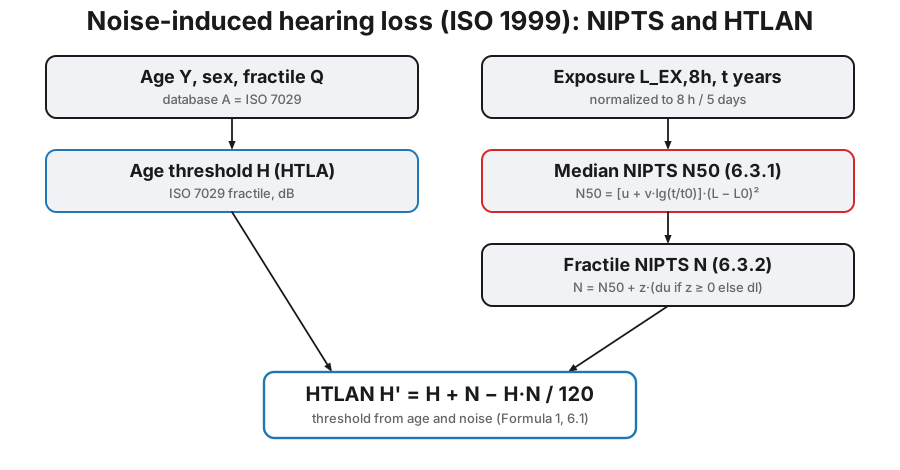
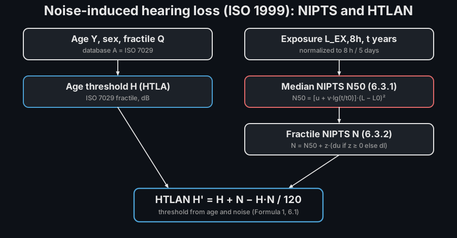
ISO 1999:2013 estimates the hearing loss a population suffers from occupational noise. It gives the noise-induced permanent threshold shift (NIPTS), the extra hearing loss caused by the noise, on top of ageing, as a function of the exposure level, the exposure duration and the audiometric frequency, together with its spread across a population. It then combines the noise component with the age component (the ISO 7029 threshold, “database A”) into the hearing threshold level associated with age and noise (HTLAN). Both are defined at the six audiometric frequencies 500 Hz to 6000 Hz, where noise damage concentrates (the characteristic 4 kHz notch).

1. Noise-induced permanent threshold shift (clause 6.3)

The median NIPTS for exposure durations of 10 to 40 years grows with the square of the excess of the noise exposure level over a frequency-dependent cut-off $L_0$ (ISO 1999 clause 6.3.1, Formula 2, Table 1):

$$N_{50}=\left[u+v\lg \frac{t}{t_0}\right](L_{EX,8h}-L_0{)}^2,$$

with $t$ the exposure in years and $t_0=1$ year; below $L_0$ the effect is zero. A population fractile follows from two half-Gaussians whose spreads $d_u$ (worse than the median) and $d_l$ (better) are given by Formulae 6/7 and Table 3: $N_{50}+zd$ with $z$ the standard-normal quantile, clamped at zero (clause 6.3.2).

The fractile argument is the fraction of the population below the returned value, so fractile=0.9 is the most-susceptible tenth. Note that ISO 1999 writes its own percentage $Q$ the other way round: in Formulae (4)/(5) $Q$ is the percentage with worse hearing, so that same tenth is $Q=10\%$, which is how the .report() fiche prints it and how the Annex D columns are headed.

from phonometry import hearing

# Median NIPTS after 20 years at an 8 h-normalised level of 90 dB(A).
r = hearing.nipts(90.0, 20.0, fractile=0.5)
print(r.frequencies.astype(int))  # [ 500 1000 2000 3000 4000 6000]
print(r.median.round(1))          # [ 0.   0.1  4.1 10.2 12.9  8.5]

# The most-susceptible tenth of the population (90th percentile):
print(hearing.nipts(90.0, 20.0, fractile=0.9).value.round(1))
# [ 0.   0.1  7.7 16.2 17.8 13.6]

r.plot()   # the NIPTS spectrum with its fractile band (needs matplotlib)

The shift peaks near 4 kHz and deepens with both level and duration. Below the cut-off (here 500 Hz, $L_0=93$ dB, and 1000 Hz, $L_0=89$ dB, at 90 dB) the noise causes no permanent shift. For durations under 10 years the median is extrapolated from the 10-year value (Formula 3); a subset of the frequencies can be requested with frequencies=.

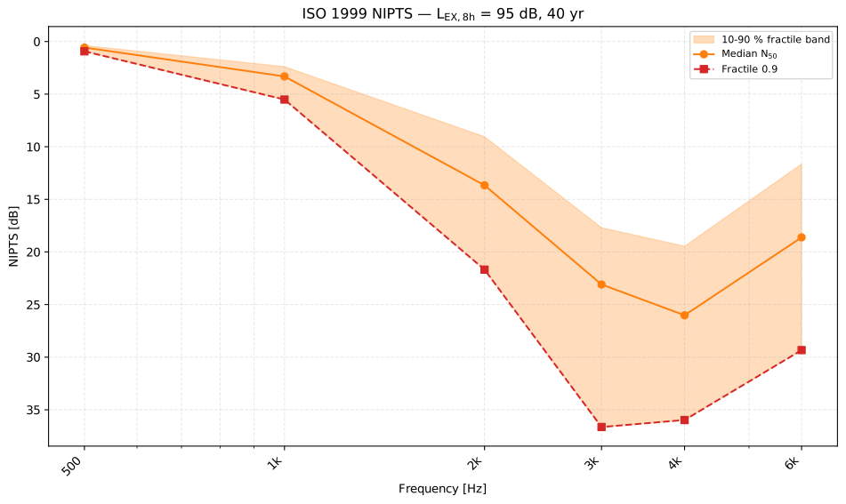
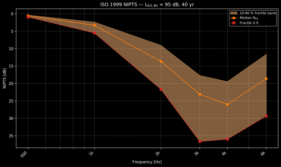
A longer, louder career makes the shape unmistakable:

Show the code for this figure

import matplotlib.pyplot as plt
from phonometry import hearing

# 40 years at an 8 h-normalised 95 dB(A), most-susceptible tenth.
res = hearing.nipts(95.0, 40.0, fractile=0.9)
print(res.median.round(1))    # the median N50
print(res.value.round(1))     # the 90 % fractile

# One line: the median, the fractile and the 10-90 % band.
res.plot()
plt.show()

The notch at 3 kHz to 4 kHz, with partial recovery at 6 kHz, is the signature of noise damage and the reason audiometric surveillance tests those frequencies. It comes out of the model rather than being imposed on it: the cut-off level $L_0$ and the coefficients $u$, $v$ of Table 1 are lowest where the ear is most vulnerable, so the same $L_{EX,8h}$ buys far more shift at 4 kHz than at 500 Hz.

2. Age and noise combined: HTLAN (clause 6.1)

The noise component does not simply add to the age component: ISO 1999 Formula (1) combines them with a compression term that matters once the total exceeds about 40 dB:

$$H^{\prime }=H+N-\frac{HN}{120},$$

where $H$ is the age threshold (HTLA, from ISO 7029 at the same fractile) and $N$ the NIPTS. htlan evaluates both components and their combination.

from phonometry import hearing

# A 60-year-old man, 30 years at 95 dB(A), median.
h = hearing.htlan(60, "male", 95.0, 30.0, fractile=0.5)
print(h.htla.round(1))       # [ 6.   7.8 12.5 16.6 20.2 25.9]  age alone
print(h.nipts.round(1))      # [ 0.5  3.  11.8 21.6 24.8 17.6]  noise alone
print(h.threshold.round(1))  # [ 6.5 10.7 23.  35.2 40.8 39.8]  age + noise

h.plot()   # the three curves of the figure below: HTLA, NIPTS and HTLAN

At 4 kHz the age component (20.2 dB) and the noise component (24.8 dB) combine to 40.8 dB rather than their 45.0 dB sum; the compression term removes 4.2 dB.

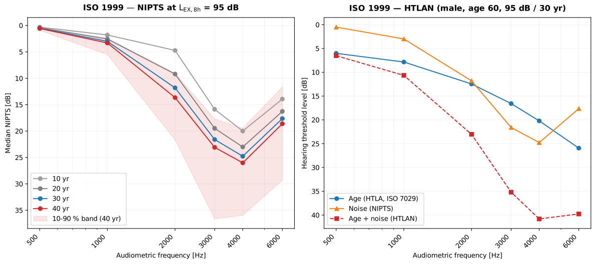
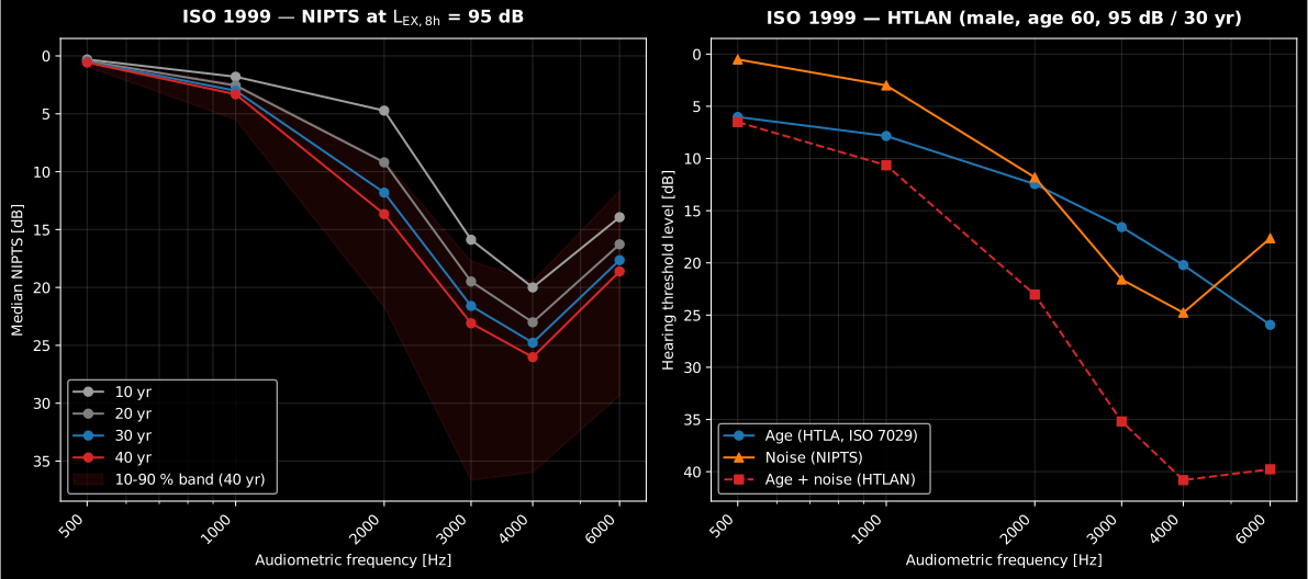
Show the code for this figure

import matplotlib.pyplot as plt
from phonometry import hearing
from phonometry.hearing.noise_induced_hearing_loss import NIPTS_FREQUENCIES as f

# One line for the NIPTS spectrum with its fractile band:
hearing.nipts(95.0, 40.0, 0.9).plot()
plt.show()

# By hand, both panels:
fig, (ax1, ax2) = plt.subplots(1, 2, figsize=(12.5, 5.6))
for yr in (10, 20, 30, 40):
    ax1.plot(f, hearing.nipts(95.0, yr, 0.5).median, "o-", label=f"{yr} yr")
ax1.set_xscale("log"); ax1.invert_yaxis(); ax1.legend()

h = hearing.htlan(60, "male", 95.0, 30.0, 0.5)
ax2.plot(f, h.htla, "o-", label="Age (HTLA)")
ax2.plot(f, h.nipts, "^-", label="Noise (NIPTS)")
ax2.plot(f, h.threshold, "s--", label="Age + noise (HTLAN)")
ax2.set_xscale("log"); ax2.invert_yaxis(); ax2.legend()
plt.show()

Three quantities, kept distinct. It is worth being precise about what each symbol means, because they are easy to conflate:

• NIPTS ($N$) is the noise-induced permanent threshold shift: the extra loss the noise causes, and nothing else. It is what an ideal hearing- conservation programme would prevent. On its own it is not an audiogram.
• HTLA ($H$) is the age threshold alone (the ISO 7029 component of the hearing-threshold guide), the loss the same person would have with no occupational noise.
• HTLAN ($H^{\prime }$) is the total threshold: age and noise combined by Formula (1). This is what an audiometer measures, and the only one of the three you can compare against a real audiogram.

The non-linear combination $H^{\prime }=H+N-HN/120$ is why you cannot simply read NIPTS off a measured audiogram by subtracting an age table: near-total losses would otherwise exceed the ~120 dB physiological ceiling, so the standard compresses the sum. Because the correction $HN/120$ scales with the product of the two components, it can already shave a few dB while $H+N$ is below 40 dB; 40 dB is only a rough marker for where the effect becomes noticeable, not a hard boundary, and the correction grows steadily in the regime of a long, loud exposure where both terms are large.

Fence caveats. ISO 1999 gives thresholds and their distribution; it does not define a “hearing handicap” or a compensable fence. A fence is a policy line (commonly a 25 dB average over selected frequencies) above which hearing is deemed impaired, and it lives in national regulation, not in this standard. Two cautions follow. First, the fence frequencies matter: averaging over 0.5/1/2 kHz (a classic speech fence) barely sees the 3–6 kHz noise notch, so it under-reports early noise damage that a 3/4/6 kHz average would catch. Second, NIPTS and HTLAN answer different fence questions: NIPTS asks “how much did the noise add”, HTLAN “is this ear, age included, over the line”; and a population’s percentage beyond fence depends on the fractile spread, not just the median, so it must be read from the distribution, never from the median threshold alone.

The NiptsResult carries the median (N50), the spread_upper/spread_lower and the value at the requested fractile; the HtlanResult carries htla, nipts and the combined threshold. Both expose .plot(). The age component alone is the subject of the hearing-threshold guide.

What this guide covers

Covered. ISO 1999:2013 as implemented by nipts and htlan: the median NIPTS of clause 6.3.1 (Formula 2, extrapolated below 10 years by Formula 3, Table 1) and its population fractile of clause 6.3.2 (Formulae 4-7, Tables 2-3), together with the HTLAN combination of clause 6.1 (Formula 1) run by combine_age_and_noise, all validated against the Annex D worked examples. The age component is database A, evaluated from ISO 7029:2017, the edition clause 6.2.2 references undated.

Not covered. Clauses 6.2.3 and 6.2.4 let the user substitute a database B for database A: an age threshold measured on a control population of the country under consideration. Only database A is implemented, so htlan always draws its age component from ISO 7029:2017. combine_age_and_noise accepts an external HTLA array for that case, but computing database B itself is not phonometry’s job. ISO 1999 does not define a “hearing handicap” or a compensable fence: that line is set by national regulation, and nothing here applies one, so you must supply and check it yourself.

See also

• API reference: hearing.noise_induced_hearing_loss.

References

• International Organization for Standardization. (2013). Acoustics — Estimation of noise-induced hearing loss (ISO 1999:2013). The implemented model: the HTLAN combination (clause 6.1, Formula 1), the median NIPTS (clause 6.3.1, Formulae 2-3, Table 1) and its statistical distribution (clause 6.3.2, Formulae 4-7, Tables 2-3), validated against the worked examples of Annex D. The age component (database A) is ISO 7029:2017.
• National Institute for Occupational Safety and Health. (1998). Criteria for a recommended standard: Occupational noise exposure — Revised criteria 1998 (DHHS/NIOSH Publication No. 98-126). https://doi.org/10.26616/NIOSHPUB98126A freely available criteria document (the linked PDF is the free download) reviewing the same exposure-response evidence and the fence and hearing-conservation issues discussed on this page.
• Passchier-Vermeer, W. (1974). Hearing loss due to continuous exposure to steady-state broad-band noise. The Journal of the Acoustical Society of America, 56(5), 1585-1593. https://doi.org/10.1121/1.1903482One of the field studies whose exposure-response data underpin the NIPTS relations later codified in ISO 1999.