Objective Intelligibility (STOI & ESTOI)

STOI and ESTOI are correlation-based objective intelligibility measures. Each compares a clean reference to a degraded or processed version of the same speech and returns a scalar with a monotonic relation to the fraction of words a listener would understand: 1 when the degraded signal equals the clean one, and near 0 for uncorrelated noise. They work directly on the two waveforms, which makes them the standard yardstick for time-frequency weighted speech: noise reduction, source separation and binary-mask processing, where separating the clean speech from its distortion is not straightforward.

Note

STOI/ESTOI vs STI vs SII. STOI and ESTOI need the clean reference and the degraded signal, and rate the processing between them. The Speech Transmission Index rates a transmission channel from its impulse response, and the Speech Intelligibility Index predicts audibility from speech, noise and hearing-threshold spectra. Use STOI/ESTOI when you have a before/after pair.

Caution

pystoi (a public reimplementation of the authors’ MATLAB) is used only as an external cross-check in the test suite. phonometry reimplements both measures from the two papers and never imports pystoi at runtime; the two agree to well under 1e-3 on shared inputs.

1. The shared front end

Both measures run the same processing before they diverge (Taal et al. 2011, Section II): resampling to 10 kHz; a 256-sample (25.6 ms) Hann-windowed, 50 %-overlapping short-time transform zero-padded to 512 points; removal of the frames whose clean energy is more than 40 dB below the loudest clean frame; a 15-band one-third-octave grouping of the DFT magnitudes from a lowest centre of 150 Hz; and 384 ms (30-frame) analysis segments as the unit of comparison. The sample rate of the inputs is free, the library resamples internally.

from phonometry import stoi

d = stoi(clean, degraded, fs)          # STOI, resampled to 10 kHz internally
print(round(d.value, 3))               # a scalar in roughly [0, 1]
print(stoi(clean, clean, fs).value)    # 1.0  (a signal against itself)

2. STOI: envelope correlation with clipping

For every band and segment STOI normalises the degraded envelope to the clean one, clips it at a lower signal-to-distortion bound ($\beta =-15$ dB) so a fully degraded unit cannot drag the score below its floor, and takes the sample correlation of the two envelopes (Taal et al. 2011, Eqs. 3-6):

$$d_{j,m}=\frac{{\sum }_n(x_j(n)-{\bar{x}}_j)({\bar{y}}_j(n)-{\overline{\stackrel{ˉ}{y}}}_j)}{\Vert x_j-{\bar{x}}_j\Vert \Vert {\bar{y}}_j-{\overline{\stackrel{ˉ}{y}}}_j\Vert }.$$

The index is the average of those intermediate correlations over all bands $j$ and segments $m$ (Eq. 6). Because the normalisation divides out a per-segment gain, STOI is invariant to the overall playback level of the degraded signal, and higher SNR gives a monotonically higher score.

import numpy as np
from phonometry import stoi

fs = 10000
rng = np.random.default_rng(1)
clean = rng.standard_normal(3 * fs)
for snr_db in (-10, 0, 10, 20):
    g = 10.0 ** (-snr_db / 20.0)
    noisy = clean + g * rng.standard_normal(clean.size)
    print(snr_db, round(stoi(clean, noisy, fs).value, 3))

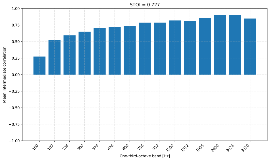
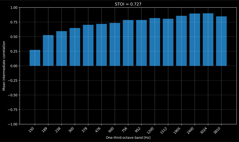
The STOIResult carries the per-band mean correlation (band_scores) and the per-segment scores (segment_scores) that average to value, and its .plot() draws the per-band intermediate correlation. That per-band view is worth looking at before quoting the index: it shows where the degradation bites, which the single number cannot.

Show the code for this figure

import numpy as np
import matplotlib.pyplot as plt
from scipy.signal import butter, lfilter
from phonometry import stoi

# Speech-like material: band-limited noise with a 3.5 Hz syllabic envelope,
# in a flat masker at 0 dB SNR.
fs = 10000
rng = np.random.default_rng(11)
t = np.arange(4 * fs) / fs
b, a = butter(2, [200 / (fs / 2), 4000 / (fs / 2)], btype="band")
carrier = lfilter(b, a, rng.standard_normal(t.size))
clean = carrier * (0.15 + 0.85 * np.abs(np.sin(2 * np.pi * 3.5 * t)) ** 2)
masker = rng.standard_normal(clean.size)
gain = np.sqrt(np.mean(clean ** 2)) / np.sqrt(np.mean(masker ** 2))
res = stoi(clean, clean + gain * masker, fs)
print(round(res.value, 3))    # 0.727

# One line: the per-band intermediate correlation behind the index.
res.plot()
plt.show()

# By hand, mirroring what STOIResult.plot() draws:
pos = np.arange(res.band_scores.size)
fig, ax = plt.subplots()
ax.bar(pos, res.band_scores)
ax.set_xticks(pos)
ax.set_xticklabels([f"{f:.0f}" for f in res.band_frequencies], rotation=45, ha="right")
ax.set_xlabel("One-third-octave band [Hz]")
ax.set_ylabel("Mean intermediate correlation")
ax.set_title(f"STOI = {res.value:.3f}")
plt.show()

The flat masker costs the low bands most, because the speech spectrum falls there while the masker does not, and the correlation recovers in the consonant-bearing bands above 1 kHz. A band profile that is flat, or that collapses only in one band, points at something other than broadband noise: a notch filter, a resonance, or a processing artefact of the enhancement under test.

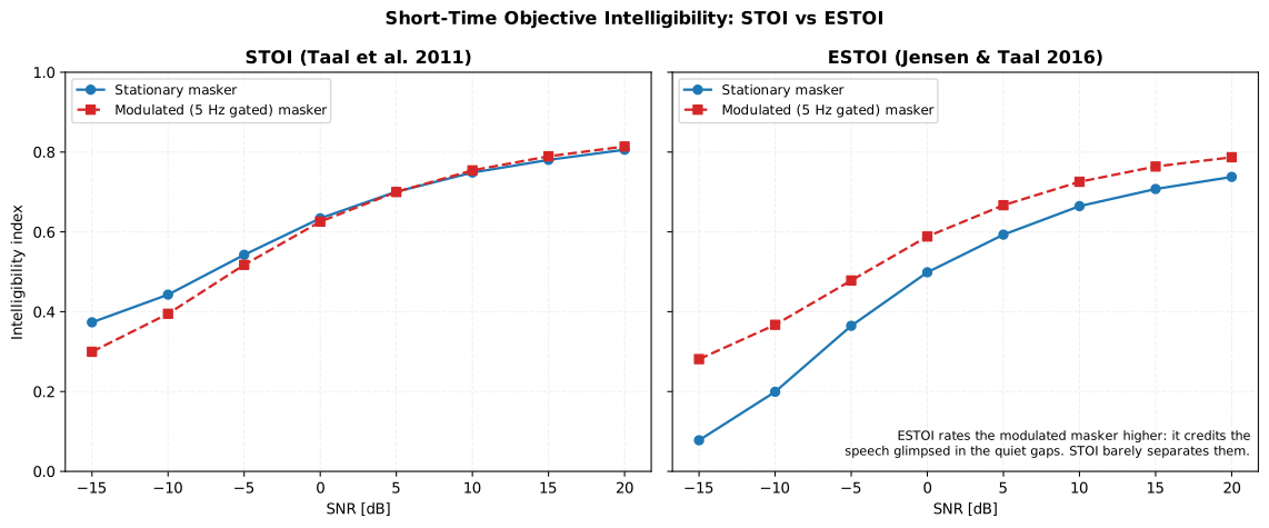
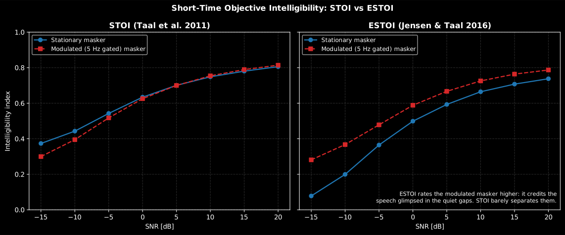
3. ESTOI: spectral correlation for modulated maskers

ESTOI (extended=True) replaces the band-independent correlation with a joint spectro-temporal one. Within each 384 ms segment it mean- and variance-normalises the spectrogram rows (the band envelopes) and then its columns (the per-frame spectra), and averages the correlation of the normalised columns (Jensen and Taal 2016, Eqs. 4-8). Making the columns compete means a masker that leaves quiet gaps, where the clean speech is briefly audible, is credited for the speech glimpsed there, which STOI’s per-band average largely misses.

Show the code for this figure

import numpy as np
import matplotlib.pyplot as plt
from phonometry import stoi

fs = 10000
rng = np.random.default_rng(20)
t = np.arange(3 * fs) / fs
# A speech-like clean signal: amplitude-modulated formant-ish tones.
clean = np.zeros_like(t)
for f0 in (200.0, 400.0, 700.0, 1100.0, 1800.0, 2600.0):
    depth = 0.5 * (1.0 + np.sin(2 * np.pi * rng.uniform(2.0, 6.0) * t + rng.uniform(0.0, 2 * np.pi)))
    clean += depth * np.sin(2 * np.pi * f0 * t + rng.uniform(0.0, 2 * np.pi))
p_clean = np.sqrt(np.mean(clean ** 2))

base = rng.standard_normal(clean.size)
gate = 0.5 * (1.0 + np.sign(np.sin(2 * np.pi * 5.0 * t)))   # 5 Hz on/off gate
modulated = base * (0.05 + 0.95 * gate)
snrs = np.arange(-15.0, 20.1, 5.0)

def curve(masker, extended):
    p_m = np.sqrt(np.mean(masker ** 2))
    return [stoi(clean, clean + (p_clean / (p_m * 10.0 ** (s / 20.0))) * masker,
                 fs, extended=extended).value for s in snrs]

fig, (a, b) = plt.subplots(1, 2, figsize=(12, 5), sharey=True)
for ax, extended, title in ((a, False, "STOI"), (b, True, "ESTOI")):
    ax.plot(snrs, curve(base, extended), "o-", label="Stationary masker")
    ax.plot(snrs, curve(modulated, extended), "s--", label="Modulated masker")
    ax.set_title(title); ax.set_xlabel("SNR [dB]"); ax.set_ylim(0, 1); ax.legend()
a.set_ylabel("Intelligibility index")
plt.show()

4. Which measure, and when

	STOI	ESTOI
Intermediate quantity	Per-band envelope correlation, clipped	Row- and column-normalised spectral correlation
Level invariance	Yes (per-segment normalisation)	Yes (per-row and per-column normalisation)
Stationary maskers	Well validated	Well validated
Modulated maskers, competing talkers	Underrates the glimpsing benefit	Tracks it
Cost	Lower	A little higher

For additive stationary noise the two measures are interchangeable and STOI is the lighter default; when the interference fluctuates in time, or when comparing processors that reshape the speech in time and frequency, prefer ESTOI.

Both answer a narrower question than the two standardised speech metrics of the library, and the choice between the three families is really a choice of what you can measure. STOI and ESTOI need a clean reference and the degraded signal, so they belong to processing work: noise reduction, source separation, codecs, hearing-aid algorithms. The STI (IEC 60268-16) needs no clean reference, only the channel, so it is what rates a room or a public-address system. The SII (ANSI S3.5-1997) needs neither signal, only spectra, so it is what predicts audibility for a listener with a given hearing threshold. When more than one is available, they answer different questions rather than confirming each other: a processor can raise STOI while the room keeps the STI poor.

What this guide covers

Covered. Taal et al. 2011 (STOI) and Jensen & Taal 2016 (ESTOI), the two correlation-based measures stoi() implements: the shared front end of 10 kHz resampling, 256-sample Hann frames, 15 one-third-octave bands, 384 ms segments and 40 dB silent-frame removal (Taal et al. 2011, Eqs. 1-4); the per-band envelope correlation and averaged index (Eqs. 5-6); and, with extended=True, the row- and column-normalisation of the spectrogram and the spectral-correlation index (Jensen & Taal 2016, Eqs. 4-8).

Not covered. Taal et al. 2011 also fits a logistic function mapping the index $d$ to a predicted percentage of words understood, calibrated on specific listening-test corpora. stoi() returns only $d$, as STOIResult.value, not that percentage: the API has no percent-correct output or fitted coefficients. The 2010 ICASSP paper is cited only as the short conference version of the same algorithm, adding nothing implemented beyond the 2011/2016 equations above.

See also

• Speech Transmission Index: rates a transmission channel from its impulse response or a STIPA recording.
• Speech Intelligibility Index: predicts intelligibility from speech, noise and hearing-threshold spectra.
• Filter Banks: the one-third-octave bands the front end groups the DFT into.
• API reference: hearing.objective_intelligibility.

References

• Jensen, J., & Taal, C. H. (2016). An algorithm for predicting the intelligibility of speech masked by modulated noise maskers. IEEE/ACM Transactions on Audio, Speech, and Language Processing, 24(11), 2009-2022. https://doi.org/10.1109/TASLP.2016.2585878ESTOI: the row- and column mean- and variance-normalisation of the short-time spectrogram (Eqs. 4-7) and the spectral-correlation intermediate index (Eq. 8).
• Taal, C. H., Hendriks, R. C., Heusdens, R., & Jensen, J. (2010). A short-time objective intelligibility measure for time-frequency weighted noisy speech. 2010 IEEE International Conference on Acoustics, Speech and Signal Processing (ICASSP), 4214-4217. https://doi.org/10.1109/ICASSP.2010.5495701The short conference version of STOI.
• Taal, C. H., Hendriks, R. C., Heusdens, R., & Jensen, J. (2011). An algorithm for intelligibility prediction of time-frequency weighted noisy speech. IEEE Transactions on Audio, Speech, and Language Processing, 19(7), 2125-2136. https://doi.org/10.1109/TASL.2011.2114881STOI: the shared front end (10 kHz, 256-sample Hann frames, 15 one-third-octave bands, 384 ms segments), the normalisation and signal-to-distortion clipping (Eqs. 1-4), the per-band envelope correlation (Eq. 5) and the averaged index (Eq. 6).