Measurement uncertainty (GUM and Monte Carlo)

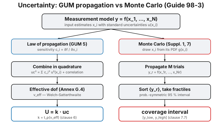
Every measurement result is incomplete without a statement of its uncertainty. The Guide to the Expression of Uncertainty in Measurement gives two ways to propagate the uncertainties of the inputs of a measurement model $y=f(x_1,\dots ,x_N)$ to the output: the law of propagation of uncertainty (ISO/IEC Guide 98-3:2008, the GUM, clause 5) and the Monte Carlo method (ISO/IEC Guide 98-3-1:2008, Supplement 1, clause 7). The first combines standard uncertainties analytically through the sensitivity coefficients; the second propagates the whole probability distributions numerically. They agree for linear models and diverge, informatively, when the model is non-linear or the inputs are far from Gaussian.

1. The law of propagation of uncertainty (GUM clause 5)

For a model $y=f(x_1,\dots ,x_N)$ with uncorrelated inputs, the combined standard uncertainty is the quadrature sum of the input contributions $u_i(y)=|c_i|u(x_i)$ weighted by the sensitivity coefficients $c_i=\partial f/\partial x_i$:

$$u_c^2(y)=\sum _{i=1}^N{\left(\frac{\partial f}{\partial x_i}\right)}^2{u}^2(x_i).$$

combine_uncertainty evaluates the sensitivities by central differences, so any callable model works, with no hand-derived partials. Input quantities are described by a Quantity (best estimate, standard uncertainty, PDF, degrees of freedom). Type B evaluations from a half-width $a$ are built by rectangular ($a/\sqrt{3}$), triangular ($a/\sqrt{6}$) and u_shaped ($a/\sqrt{2}$) (GUM clause 4.3).

from phonometry import metrology

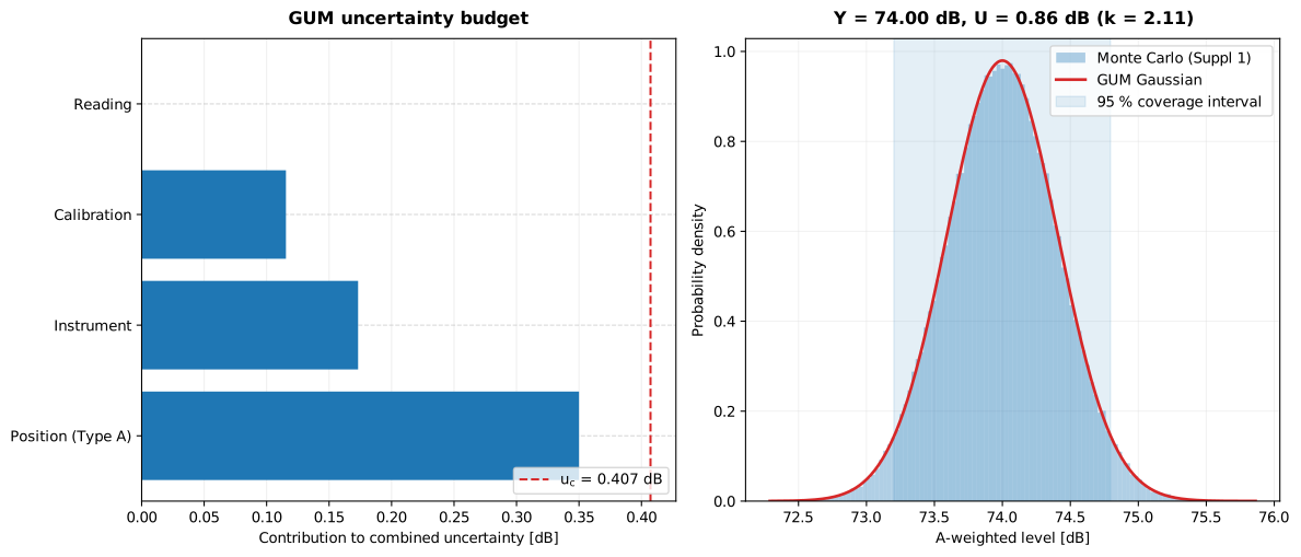
# A-weighted level: a reading plus zero-mean calibration, instrument and
# positional corrections. The model is their sum.
quantities = [
    metrology.Quantity(74.0, 0.0, name="Reading"),
    metrology.rectangular(0.0, 0.20, name="Calibration"),
    metrology.rectangular(0.0, 0.30, name="Instrument"),
    metrology.Quantity(0.0, 0.35, dof=9, name="Position (Type A)"),
]
result = metrology.combine_uncertainty(lambda a, b, c, d: a + b + c + d, quantities)

print(round(result.value, 2))                 # 74.0
print(round(result.combined_uncertainty, 3))  # 0.407 dB
print(result.contributions.round(3))          # [0.    0.115 0.173 0.35 ]
print(round(result.effective_dof, 1))         # 16.5

k, U = result.expanded(0.95)
print(round(k, 2), round(U, 2))               # 2.11 0.86  ->  Y = 74.0 ± 0.9 dB

The expanded uncertainty $U=k{u}_c$ scales the combined uncertainty by a coverage factor $k=t_p({\nu }_{\text{eff}})$ from the $t$-distribution at the effective degrees of freedom given by the Welch–Satterthwaite formula (Annex G.4). Here the single Type A input (9 degrees of freedom) pulls ${\nu }_{\text{eff}}$ down to about 16, so $k=2.11$ rather than the large-sample 1.96. Correlated inputs are handled by passing a correlation matrix; a fully correlated sum then adds linearly instead of in quadrature. Correlation is the classic silent error in a budget: two corrections traceable to the same calibrator, or two channels sharing one instrument, do not average away the way independent terms would, and combining them in quadrature as if they were uncorrelated typically understates $u_c$ (with sensitivities of opposite sign the bias can point the other way). Because the GUM defines Welch–Satterthwaite for independent inputs only, a correlated budget with finite input degrees of freedom carries no effective degrees of freedom at all: effective_dof is NaN, a warning is issued, and expanded() requires an explicit coverage_factor_override (e.g. $k=2$) rather than inventing one. Only when every input is Type B with infinite degrees of freedom does a correlated budget keep ${\nu }_{\text{eff}}=\infty$ and use the normal-distribution coverage factor. This chain reproduces the GUM’s own worked examples end to end: the Annex H.1 end-gauge budget ($u_c=31.7$ nm, $U_{99}=92$ nm against the printed 32/93) and the Annex H.2 correlated resistance measurement ($u_c(R)=0.071\Omega$, $u_c(X)=0.295\Omega$, $u_c(Z)=0.236\Omega$ from Table H.3).

2. The Monte Carlo method (Supplement 1)

When the model is non-linear or the inputs are markedly non-Gaussian, the GUM Gaussian assumption for the output can be inaccurate. monte_carlo instead draws samples of each input from its PDF, evaluates the model over all trials and reports the mean, the standard deviation and the probabilistically symmetric coverage interval (equal probability in each tail, clause 7.7). The inputs are sampled independently; the Supplement’s multivariate-Gaussian path for non-independent quantities (6.4.8) is not implemented, so correlated budgets belong to combine_uncertainty. The number of trials is fixed (no adaptive 7.9 procedure, at least 2 trials) and the interval is the symmetric one, not the 5.3.4 shortest interval.

from phonometry import metrology

quantities = [
    metrology.Quantity(74.0, 0.0, name="Reading"),
    metrology.rectangular(0.0, 0.20, name="Calibration"),
    metrology.rectangular(0.0, 0.30, name="Instrument"),
    metrology.Quantity(0.0, 0.35, dof=9, name="Position (Type A)"),
]
mc = metrology.monte_carlo(lambda a, b, c, d: a + b + c + d, quantities,
                    trials=1_000_000, coverage=0.95, seed=1)

print(round(mc.value, 2))                 # 74.0
print(round(mc.standard_uncertainty, 3))  # 0.407 dB  (matches uc above)
print([round(x, 2) for x in mc.interval]) # [73.2, 74.8]

For this near-linear model the Monte Carlo standard uncertainty reproduces the GUM $u_c$ to three digits and the 95 % interval matches $Y\pm U$. The two methods are validated against the Guides’ own worked examples: the additive model of four unit inputs gives $u_c=2.0$ (Supplement 1 clause 9.2), and four rectangular inputs give a Monte Carlo interval of $[-3.88,3.88]$ (Supplement 1 clause 9.2.3).

When does the Monte Carlo method earn its extra cost? Whenever either of the GUM’s two simplifications fails: the model is replaced by its first-order expansion, and the output distribution by a Gaussian (or a $t$). Both hold well for the additive level model above, which is why the two methods agree to three digits. They stop holding when the model is strongly non-linear over the span of the input uncertainties (energy-to-level conversions with wide inputs, products and quotients with large relative uncertainties), when a single non-Gaussian input dominates the budget (one large rectangular term makes the output nearly rectangular, and a Gaussian $\pm 2u_c$ interval overcovers it), or when the output sits near a physical bound (an absorption coefficient near 0 or 1, a level correction that cannot cross zero), where the true coverage interval is asymmetric and no $Y\pm U$ statement can represent it. In those regimes the Monte Carlo interval is the reference: Supplement 1 (clause 8) treats the GUM framework as validated precisely when it agrees with the Monte Carlo result, and as superseded by it when it does not.

Show the code for this figure

import matplotlib.pyplot as plt
import numpy as np
from phonometry import metrology

quantities = [
    metrology.Quantity(74.0, 0.0, name="Reading"),
    metrology.rectangular(0.0, 0.20, name="Calibration"),
    metrology.rectangular(0.0, 0.30, name="Instrument"),
    metrology.Quantity(0.0, 0.35, dof=9, name="Position (Type A)"),
]
model = lambda a, b, c, d: a + b + c + d
result = metrology.combine_uncertainty(model, quantities)
mc = metrology.monte_carlo(model, quantities, trials=1_000_000, coverage=0.95, seed=1,
                    keep_samples=True)
k, U = result.expanded(0.95)

# One line per panel — the budget bars, and the Monte Carlo histogram with
# its coverage interval (the committed figure also overlays the GUM Gaussian):
result.plot()
mc.plot()
plt.show()

# By hand, both panels — budget bars and the Monte Carlo output distribution:
fig, (ax1, ax2) = plt.subplots(1, 2, figsize=(12.5, 5.4))
ax1.barh(result.names, result.contributions)
ax1.axvline(result.combined_uncertainty, ls="--",
            label=f"$u_c$ = {result.combined_uncertainty:.3f} dB")
ax1.invert_yaxis(); ax1.legend()

rng = np.random.default_rng(1)
samples = model(np.full(200_000, 74.0),
                rng.uniform(-0.20, 0.20, 200_000),
                rng.uniform(-0.30, 0.30, 200_000),
                rng.normal(0.0, 0.35, 200_000))
ax2.hist(samples, bins=120, density=True, alpha=0.35, label="Monte Carlo")
ax2.axvspan(*mc.interval, alpha=0.12, label="95 % coverage interval")
ax2.set_title(f"Y = {result.value:.2f} dB,  U = {U:.2f} dB (k = {k:.2f})")
ax2.legend()
plt.show()

The UncertaintyResult carries the value, combined_uncertainty, the sensitivities, the per-input contributions and the effective_dof; its .plot() draws the budget and .expanded(coverage) returns the pair $(k,U)$. The MonteCarloResult carries the value, standard_uncertainty, the coverage interval and its coverage; with keep_samples=True it also retains the output samples, and its .plot() draws the output histogram with the coverage interval marked (the right panel above). The building-acoustics uncertainty of ISO 12999-1, which combines reproducibility terms for a single-number rating, is a separate, domain-specific budget.

A budget is only as honest as the record behind it: every averaged input assumes stationarity, and Data qualification provides the Bendat & Piersol tests that check it before the propagation starts.

Where the library consumes this machinery

The domain pages carry their own, standard-prescribed uncertainty clauses, and each is an instance of the clause-5 sum this page implements in general form; use this page whenever your measurement model is not one of those standardized cases:

• Calibration. The calibrator’s class tolerance and the pre/post drift bound of Calibration are textbook Type B inputs: propagate them (Quantity(..., "rectangular")) through the level model rather than quoting the tolerance alone.
• Environmental levels. The ISO 1996-2 combined uncertainty of the Levels page is Formula (2) of that standard: the same quadrature sum with the standard’s own sensitivity coefficients.
• Building acoustics. The per-band and single-number uncertainties of field insulation measurements apply the tabulated reproducibility terms of ISO 12999-1, a standardized budget for one specific model.
• Absorption. The materials page carries the ISO 12999-2 absorption uncertainty, the same construction for the reverberation-room method.
• Occupational exposure. The ISO 9612 uncertainty of occupational measurements budgets sampling, instrument and position contributions in exactly this way.

See also

• Data qualification: the stationarity checks every averaged input silently assumes.
• Calibration: the tolerance and drift inputs of every calibrated chain.
• API reference: metrology.uncertainty.

References

• International Organization for Standardization. (2020). Acoustics — Determination and application of measurement uncertainties in building acoustics — Part 1: Sound insulation (ISO 12999-1:2020). The domain-specific reproducibility budget for building-acoustics single-number ratings, a separate companion to the general GUM machinery.
• Joint Committee for Guides in Metrology. (2008). Evaluation of measurement data — Guide to the expression of uncertainty in measurement (JCGM 100:2008, the GUM). BIPM. https://doi.org/10.59161/JCGM100-2008EThe law of propagation of uncertainty (clause 5), Type B evaluation (clause 4.3), the expanded uncertainty and coverage factor (clause 6, Annex G), the Welch–Satterthwaite effective degrees of freedom (Annex G.4) and the Annex H worked examples that section 1 implements and reproduces. Also published as ISO/IEC Guide 98-3:2008, Uncertainty of measurement — Part 3: Guide to the expression of uncertainty in measurement (GUM:1995). The linked PDF is the free download.
• Joint Committee for Guides in Metrology. (2008). Evaluation of measurement data — Supplement 1 to the "Guide to the expression of uncertainty in measurement" — Propagation of distributions using a Monte Carlo method (JCGM 101:2008). BIPM. https://doi.org/10.59161/JCGM101-2008The Monte Carlo propagation of section 2, its probabilistically symmetric coverage interval (clause 7) and the clause 8 validation of the GUM framework against the Monte Carlo result. Also published as ISO/IEC Guide 98-3-1:2008. The linked PDF is the free download.