Predicting Sound Insulation (EN 12354)
Standards: EN 12354Key references: Hopkins 2007
A laboratory rating describes an element in isolation; a building also transmits sound along every flanking path. This page covers the EN 12354 prediction of in-situ performance from laboratory element data: the airborne and impact flanking models of EN 12354-1/2 with their junction vibration reduction indices, and the façade insulation and outdoor radiation of EN 12354-3/4. The measured quantities the model is checked against live in Field Insulation Measurement and Ratings; the laboratory inputs come from Laboratory Insulation Measurement.
How do I predict sound insulation with EN 12354 in Python?
Section titled “How do I predict sound insulation with EN 12354 in Python?”Build the three flanking paths of each junction with
building.flanking_element(), then combine them with
building.predicted_airborne_insulation(r_direct=57.0, flanking_paths=paths).
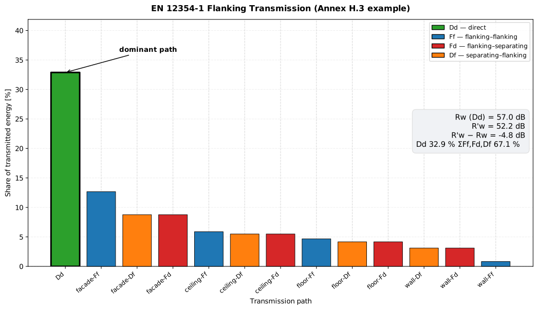
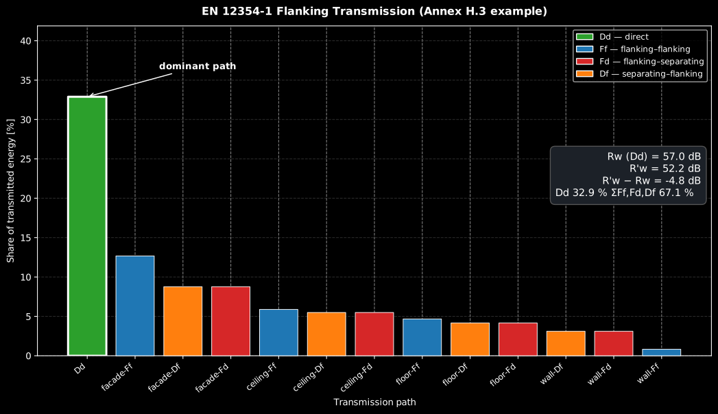
For the EN 12354-1 Annex H.3 example below it returns r_prime_w = 52.2 dB,
that is = 52 dB, and names the dominant path. Impact insulation goes
through predicted_impact_insulation().
Predicting performance (EN 12354)
Section titled “Predicting performance (EN 12354)”A laboratory rating describes an element in isolation, yet the sound a building actually transmits also travels around the partition (along the floor, up the façade, through the flanking walls), re-radiating into the receiving room. This flanking transmission is the whole difference between the laboratory and the field . EN 12354 predicts the in-situ apparent rating from the laboratory ratings of the elements plus the vibration transmission of their junctions.
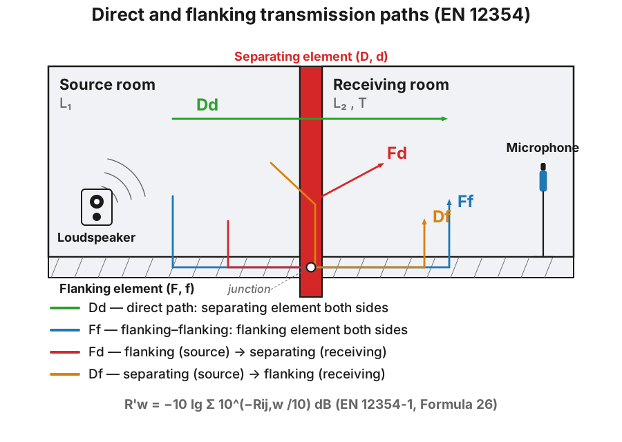
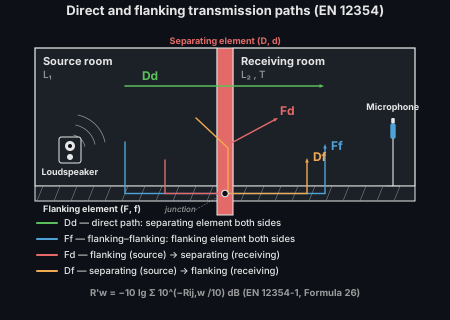
Each junction between a flanking element and the separating element carries three paths, (flanking→flanking), (direct→flanking) and (flanking→direct), alongside the single direct path .
Energy pulses leave the source room over the direct Dd path and the flanking Ff, Fd and Df paths, shrinking at each element and junction, and every path label lights up as its pulse re-radiates into the receiving room.
Energy pulses leave the source room over the direct Dd path and the flanking Ff, Fd and Df paths, shrinking at each element and junction, and every path label lights up as its pulse re-radiates into the receiving room.
The simplified single-number model combines them energetically (Formula 26):
with the direct path (Formula 27) and each flanking path (Formula 28a)
where m is the reference coupling length, the junction coupling length and the junction’s vibration reduction index (Annex E, empirical in the mass ratio ).
import numpy as npfrom phonometry import building
# EN 12354-1 Annex H.3: a separating wall Rs,w = 57 dB, area Ss = 11.5 m², with# four flanking elements. The simplified model reads each junction's Kij at# 500 Hz from the mass ratio m'perp / m' (Annex E) — here the floor's rigid# cross-junction (the mass ratio is itself rounded, hence 12.5 vs Annex 12.4):print(round(building.junction_vibration_reduction("rigid_cross", "through", 1.61), 1))  # 12.5  KFfprint(round(building.junction_vibration_reduction("rigid_cross", "corner",  1.61), 1))  #  8.9  KFd = KDf
# Build each element's three flanking paths (Ff, Df, Fd) from the Annex H# tabulated Kij, then combine the direct path Dd energetically (Formula 26).elements = [   # (name, Rw, KFf, KFd = KDf, coupling length lf)    ("floor",    49, 12.4,  8.9, 4.50),    ("ceiling",  46, 14.4,  9.2, 4.50),    ("facade",   42, 12.6,  6.7, 2.55),    ("int-wall", 33, 33.5, 15.7, 2.55),]paths = []for name, rw, k_ff, k_fd, lf in elements:    paths += building.flanking_element(label=name, r_flanking=rw, r_separating=57,                              k_ff=k_ff, k_fd=k_fd, k_df=k_fd,                              separating_area=11.5, coupling_length=lf)
res = building.predicted_airborne_insulation(r_direct=57.0, flanking_paths=paths)print(round(res.r_prime_w, 1))                          # 52.2  ->  R'w = 52 dBprint(res.dominant.label, round(res.dominant.fraction, 2))   # Dd 0.33 (direct dominates)
res.plot()   # per-path share of the transmitted energy, largest first (needs matplotlib)
Show the code for this figure
import matplotlib.pyplot as pltfrom phonometry import building
# Build each element's three flanking paths (Ff, Df, Fd) from the Annex H# tabulated Kij, then combine the direct path Dd energetically (Formula 26).elements = [   # (name, Rw, KFf, KFd = KDf, coupling length lf)    ("floor",    49, 12.4,  8.9, 4.50),    ("ceiling",  46, 14.4,  9.2, 4.50),    ("facade",   42, 12.6,  6.7, 2.55),    ("int-wall", 33, 33.5, 15.7, 2.55),]paths = []for name, rw, k_ff, k_fd, lf in elements:    paths += building.flanking_element(label=name, r_flanking=rw, r_separating=57,                              k_ff=k_ff, k_fd=k_fd, k_df=k_fd,                              separating_area=11.5, coupling_length=lf)res = building.predicted_airborne_insulation(r_direct=57.0, flanking_paths=paths)
# Per-path sound reduction index and each path's share of the transmitted# energy for the Annex H.3 result computed above.labels = [p.label for p in res.paths]r_w = [p.r_w for p in res.paths]frac = [100.0 * p.fraction for p in res.paths]
fig, (ax1, ax2) = plt.subplots(2, 1, figsize=(9, 6), sharex=True)ax1.bar(labels, r_w, color="tab:blue")ax1.axhline(res.r_prime_w, ls="--", color="k", label=f"R'w = {res.r_prime_w:.1f} dB")ax1.set_ylabel("Path Rij,w [dB]"); ax1.legend()ax2.bar(labels, frac, color="tab:orange")ax2.set_ylabel("Energy share [%]"); ax2.set_xlabel("Transmission path")for ax in (ax1, ax2):    ax.tick_params(axis="x", rotation=45)fig.suptitle("EN 12354-1 Annex H.3 — flanking transmission")fig.tight_layout()plt.show()
Every added flanking path strictly lowers below the direct ;
res.paths exposes each path’s share of the transmitted energy so the dominant
path is visible. flanking_element is a convenience that builds one junction’s
three paths at once; the single-path constructor behind it, flanking_path,
builds one Ff, Df or Fd path at a time (Formula 28a). Clause 4.4.2 also
enforces a floor from the junction geometry
(Formula 29). Pass the flanking-element area to
flanking_element(..., flanking_area=...) and the clamp is applied
automatically per path; or compute the floor yourself with
junction_min_vibration_reduction and pass it to
flanking_path(..., kij_min=...), which raises a below-floor to the
minimum:
from phonometry import building# Kij,min = 10 lg[lf·l0·(1/Si + 1/Sj)]; large elements give a low (here negative)# floor, so a realistic tabulated Kij is rarely clamped; but small, light# elements can push it above the tabulated value (e.g. lf = 4 m, S = 1.5 m²# gives 7.3 dB, over the 5 dB lightweight floor).print(round(building.junction_min_vibration_reduction(coupling_length=4.5, s_i=11.5, s_j=11.5), 1)) # -1.1The impact counterpart (EN 12354-2, Formula 21) is a direct subtraction: , with the bare-floor equivalent level (Annex B), the covering improvement (ISO 717-2) and the flanking correction from Table 1.
from phonometry import building
# EN 12354-2 Annex E.3: a 0.14 m concrete floor (m' = 322 kg/m²) with a floating# floor (ΔLw = 33 dB), rooms one above the other, mean flanking mass 145 kg/m².ln_eq = building.equivalent_impact_level(322.0)                   # 164 - 35 lg(m')k = building.impact_flanking_correction(322.0, 145.0)             # Table 1 (sep 322, flk 145)imp = building.predicted_impact_insulation(ln_w_eq=ln_eq, delta_l_w=33.0, k_correction=k)print(round(ln_eq, 1), k, round(imp.l_prime_n_w, 1))     # 76.2 2 45.2  ->  L'n,w = 45 dB
# Exact Formula (3): L'nT,w = L'n,w - 10 lg(0.032 V). Annex E.3's own rounding# of the factor to 10 lg(V/30) sits 0.18 dB below; both give L'nT,w = 43 dB.print(round(building.standardized_impact_level(imp.l_prime_n_w, 50.0), 1))   # 43.2  L'nT,w
imp.plot()   # the Formula (21) terms as bars: Ln,w,eq - dLw + K -> L'n,w (needs matplotlib)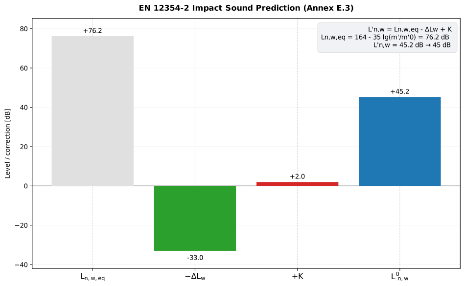
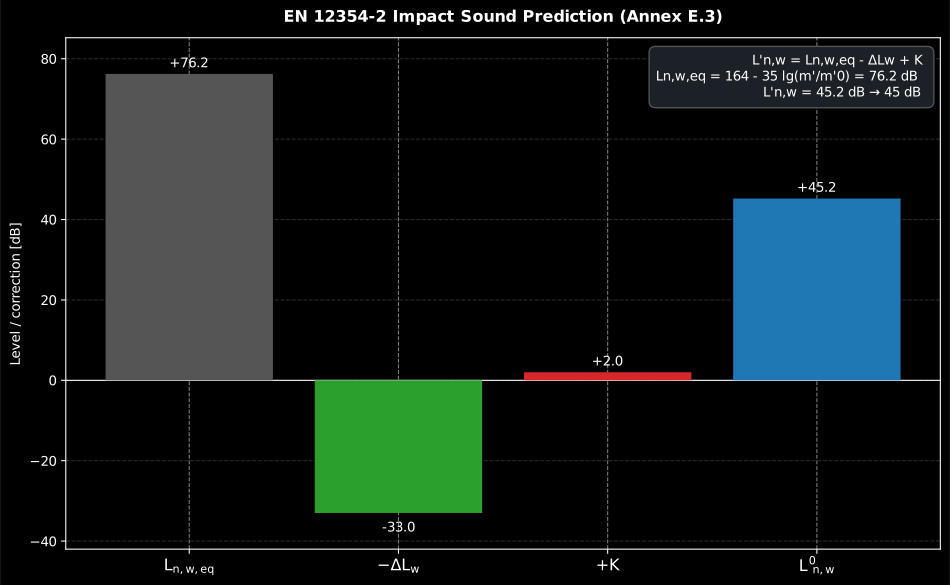
The whole EN 12354-2 simplified model is one subtraction: the massive bare floor starts at dB, the floating floor buys back 33 dB, and the flanking correction returns 2 dB, landing at dB.
Show the code for this figure
import matplotlib.pyplot as pltimport numpy as npfrom phonometry import building
# EN 12354-2 Annex E.3: 0.14 m concrete floor (m' = 322 kg/m2), floating# floor delta-Lw = 33 dB, mean flanking mass 145 kg/m2.ln_eq = building.equivalent_impact_level(322.0)k = building.impact_flanking_correction(322.0, 145.0)imp = building.predicted_impact_insulation(ln_w_eq=ln_eq, delta_l_w=33.0,                                           k_correction=k)
# One line — the Formula (21) terms as bars:imp.plot()plt.show()
# By hand, from the result's fields:labels = ["Ln,w,eq", "-dLw", "+K", "L'n,w"]values = [imp.ln_w_eq, -imp.delta_l_w, imp.k_correction, imp.l_prime_n_w]fig, ax = plt.subplots()ax.bar(np.arange(4), values)ax.axhline(0.0, color="k", lw=0.8)ax.set_xticks(np.arange(4), labels)ax.set_ylabel("Level / correction [dB]")ax.set_title(f"L'n,w = {imp.l_prime_n_w:.1f} dB (EN 12354-2 Annex E.3)")plt.show()
The airborne counterpart of that closure is Formula (5b),
, exposed as standardized_level_difference;
it closes the Annex H.3 example (standardized_level_difference(52.2, 50.0, 11.5) gives 53.6 dB, the printed chain 53.8 dB, both rounding to
dB).
The three insulation guides close a loop: the laboratory measures and element by element and junction by junction, this model assembles them into a predicted , and the field measurement checks the built result. When the measured value lands well below the prediction, look for a construction defect on the dominant path the model reports: a rigid bridge across a resilient junction, a missing lining, a leak around the separating element.
junction_vibration_reduction() / flanking_element() parameters
Section titled “junction_vibration_reduction() / flanking_element() parameters”| Parameter | Type | Units | Range / default | Notes |
|---|---|---|---|---|
junction_type | str | — | 'rigid_cross' / 'rigid_t' / 'flexible_t' / 'lightweight_facade' / 'lightweight_double_homogeneous' / 'lightweight_double_coupled' / 'corner' / 'thickness_change' | Junction geometry (Annex E.3-E.9) |
path | str | — | 'through' (K13) / 'corner' (K12 = K23) / 'double_leaf' (K24) | Path branch |
mass_ratio | float | — | > 0 | m'⊥,i / m'i (Formula E.2) |
frequency | float | Hz | default 500 | flexible_t and the E.7/E.8 double-leaf junctions are frequency-dependent |
r_flanking / r_separating | float | dB | — | Weighted indices of the flanking / separating element |
k_ff / k_fd / k_df | float | dB | — | Junction Kij for the three paths |
separating_area | float | m² | > 0 | Separating-element area Ss |
coupling_length | float | m | > 0 | Junction coupling length lf |
delta_r_ff / delta_r_fd / delta_r_df | float | dB | default 0 | Lining improvements per path |
flanking_area | float | m² | default None | Flanking-element area SF; enables the automatic Kij,min clamp (Clause 4.4.2 / Formula 29) |
flanking_path() parameters
Section titled “flanking_path() parameters”| Parameter | Type | Units | Range / default | Notes |
|---|---|---|---|---|
label | str | — | — | Display name of the path |
kind | str | — | 'Ff' / 'Df' / 'Fd' | Which flanking branch the path is |
r_source / r_receive | float | dB | — | Weighted indices of the source-side / receive-side elements |
k_ij | float | dB | — | Junction vibration-reduction index for this path |
separating_area | float | m² | > 0 | Separating-element area Ss |
coupling_length | float | m | > 0 | Junction coupling length lf |
delta_r | float | dB | default 0 | Lining improvement on this path |
kij_min | float | dB | default None | When given, k_ij is floored at this Formula (29) minimum |
predicted_airborne_insulation() returns an AirbornePredictionResult
(r_prime_w, r_direct_w, paths of PathContribution, dominant);
predicted_impact_insulation() an ImpactPredictionResult (l_prime_n_w,
ln_w_eq, delta_l_w, k_correction). The simplified model carries a reported
standard deviation of about 2 dB (Clause 5).
EN 12354 prediction report (.report())
Section titled “EN 12354 prediction report (.report())”Both prediction results write a one-page prediction report through a
report(path) method. Unlike the measurement fiches, the reported result is an
estimate of the in-situ performance from the elements’ laboratory data plus
the flanking transmission across the junctions; the sheet states this
explicitly and is labelled a prediction, never a measurement.
AirbornePredictionResult.report() renders the predicted apparent sound
reduction index fiche (the transmission-path table beside the per-path
share-of-energy plot, the boxed R'w); ImpactPredictionResult.report()
renders the predicted apparent impact-level fiche (the Formula (21) term table
beside the term plot, the boxed L'n,w). Each names EN/ISO 12354-1/-2 and the
ISO 717 rating part in its basis line, prints the model’s ~2 dB standard
deviation and, when a requirement is supplied, adds a PASS/FAIL verdict
(airborne passes at or above it, impact at or below it).
verbose=True annexes each transmission path’s share of the transmitted energy
to the airborne table. Metadata, language="es" and the phonometry[report]
extra behave exactly as in the measurement fiches; the applicable
ReportMetadata fields are the separating element (specimen), the
separating-element or floor area (area), the room geometry (source_volume,
receiving_volume), the bare floor’s mass (mass_per_area, impact), the
manufacturer (manufacturer), the test room or facility (test_room), the
calculator/laboratory identity (client, laboratory, operator,
report_id, test_date) and a free-text summary of the flanking construction
and model assumptions (notes).
from phonometry import building, ReportMetadata
# Airborne prediction (EN 12354-1 Annex H.3): a separating wall Rs,w = 57 dB# flanked by four elements -> R'w = 52 dB.paths = []for label, rw, kff, kfd, lf in [    ("floor", 49.0, 12.4, 8.9, 4.5), ("ceiling", 46.0, 14.4, 9.2, 4.5),    ("facade", 42.0, 12.6, 6.7, 2.55), ("intwall", 33.0, 33.5, 15.7, 2.55),]:    ff, df, fd = building.flanking_element(        label=label, r_flanking=rw, r_separating=57.0,        k_ff=kff, k_fd=kfd, k_df=kfd, separating_area=11.5, coupling_length=lf)    paths += [ff, df, fd]air = building.predicted_airborne_insulation(r_direct=57.0, flanking_paths=paths)air.report("Rpw_prediction.pdf", metadata=ReportMetadata(    specimen="Separating wall, Rs,w = 57 dB", area=11.5,    source_volume=53.0, receiving_volume=50.0, requirement=50.0,    notes="Flanking: floor/ceiling/facade/internal wall."))   # R'w = 52 dBair.report("Rpw_prediction_paths.pdf", verbose=True)           # + energy share
# Impact prediction (EN 12354-2 Annex E.3): a concrete floor (m' = 322 kg/m²)# with a floating floor (ΔLw = 33 dB) -> L'n,w = 45 dB.ln_eq = building.equivalent_impact_level(322.0)k = building.impact_flanking_correction(322.0, 145.0)imp = building.predicted_impact_insulation(ln_w_eq=ln_eq, delta_l_w=33.0, k_correction=k)imp.report("Lnw_prediction.pdf",           metadata=ReportMetadata(mass_per_area=322.0, requirement=53.0))  # L'n,w = 45 dB
Both example fiches are regenerated with make reports and kept rendered in
the repository; click either preview to open the PDF.
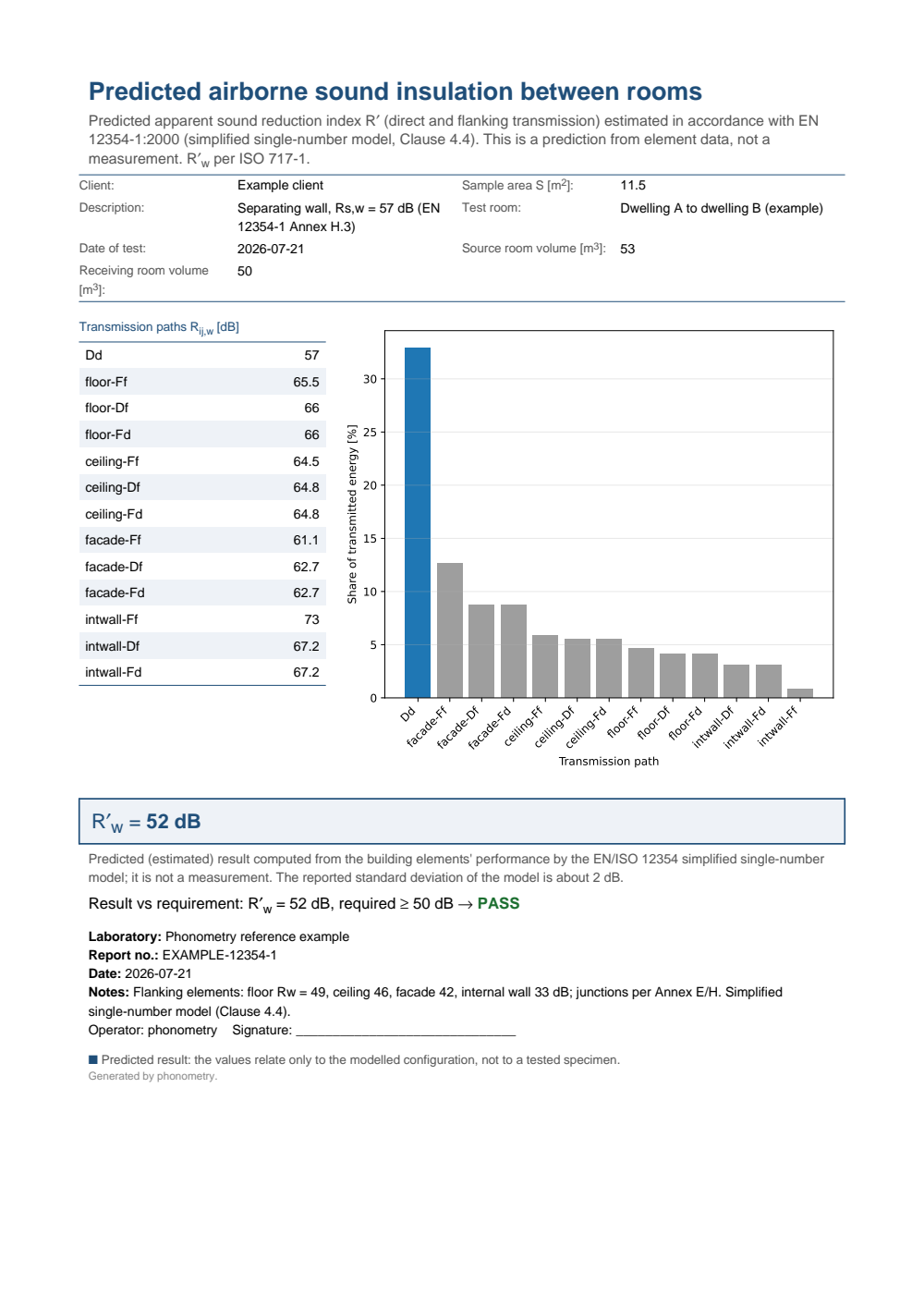
One-page predicted airborne sound insulation report between rooms (EN 12354-1 Annex H.3): the metadata header (separating element, area, room volumes), the transmission-path table (the direct path and each flanking path's weighted index Rij,w) beside the per-path share-of-energy bar chart, the boxed predicted R'w = 52 dB, the prediction statement noting the model's ~2 dB standard deviation and a PASS verdict against the 50 dB requirement.
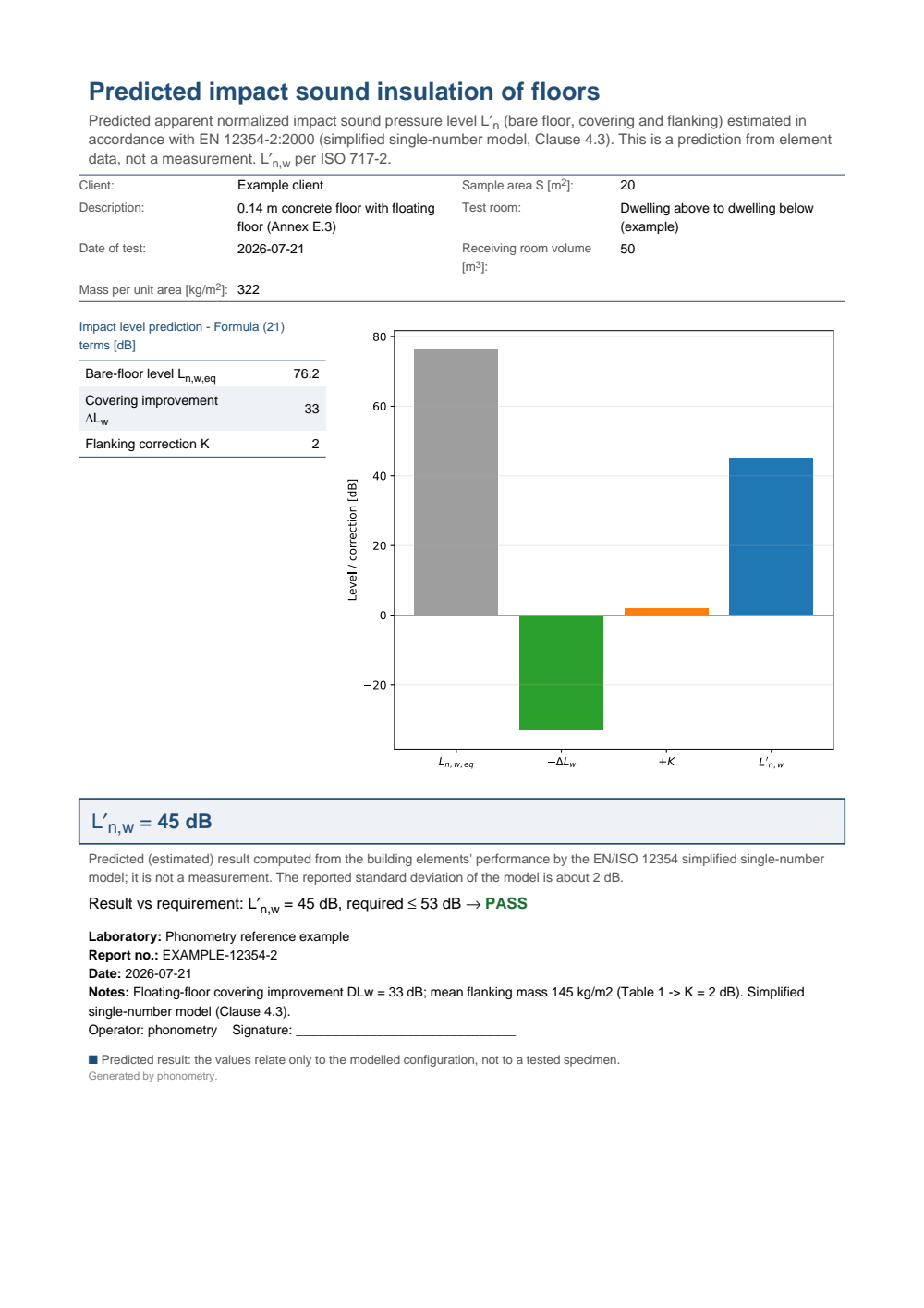
One-page predicted impact sound insulation report for a floor (EN 12354-2 Annex E.3): the metadata header, the Formula (21) term table (the bare-floor equivalent level Ln,w,eq, the covering improvement ΔLw and the flanking correction K) beside the term bar chart, the boxed predicted L'n,w = 45 dB, the prediction statement and a PASS verdict against the 53 dB requirement (a lower impact level is better).
Façade insulation & radiated power (EN 12354-3 / -4)
Section titled “Façade insulation & radiated power (EN 12354-3 / -4)”Parts 3 and 4 predict the two directions across the building envelope, both from the same energy summation of the element transmission factors , area-weighted by (a small element or air path enters through its element-normalized level difference with the reference area ):
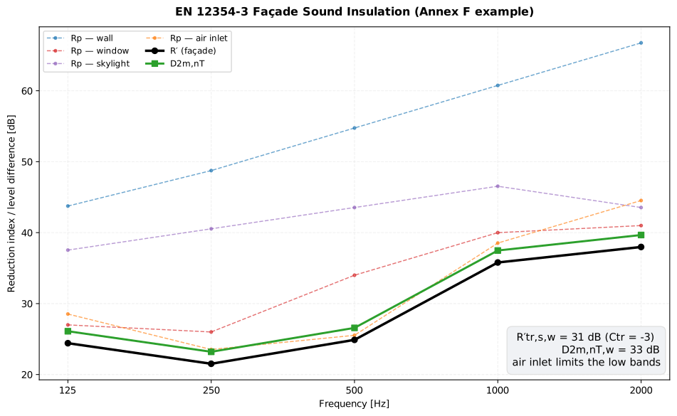
Part 3: outdoor → indoor. From (Formula 10) follow the loudspeaker- and traffic-referenced indices and , and the primary output, the standardized level difference at 2 m (Formula 13)
with the façade-shape term (Annex C; 0 dB for a flat reflecting
façade; facade_shape_level_difference looks it up from the Figure C.2 table
for galleries, balconies and terraces, interpolating over the underside
absorption ). Single-number ratings reuse EN ISO 717-1
(weighted_rating).
from phonometry import building
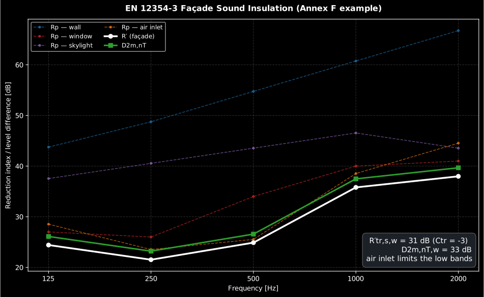
# EN 12354-3 Annex F: an 11.3 m² façade (V = 50 m³, flat so ΔLfs = 0) of a double# wall, a window, a small skylight and an acoustically-treated air inlet (a Dn,e# element).elements = [    building.FacadeElement("wall",     area=6.0, r=[41, 46, 52, 58, 64]),   # octave 125-2000    building.FacadeElement("window",   area=4.5, r=[23, 22, 30, 36, 37]),    building.FacadeElement("skylight", area=0.5, r=[24, 27, 30, 33, 30]),    building.FacadeElement("air inlet", dn_e=[28, 23, 25, 38, 44]),         # small element]fac = building.facade_sound_reduction(elements, area=11.3, volume=50.0,                             frequencies=[125, 250, 500, 1000, 2000], bands="octave")print(fac.r_tr_s_w, fac.c_tr, fac.d_2m_nt_w)   # 31 -3 33  (R'tr,s,w / Ctr / D2m,nT,w)
fac.plot()   # per-element partial indices with R' and D2m,nT overlaid (needs matplotlib)
Show the code for this figure
import numpy as npimport matplotlib.pyplot as pltfrom phonometry import building
# EN 12354-3 Annex F: an 11.3 m² façade (V = 50 m³, flat so ΔLfs = 0) of a double# wall, a window, a small skylight and an acoustically-treated air inlet (a Dn,e# element).elements = [    building.FacadeElement("wall",     area=6.0, r=[41, 46, 52, 58, 64]),   # octave 125-2000    building.FacadeElement("window",   area=4.5, r=[23, 22, 30, 36, 37]),    building.FacadeElement("skylight", area=0.5, r=[24, 27, 30, 33, 30]),    building.FacadeElement("air inlet", dn_e=[28, 23, 25, 38, 44]),         # small element]fac = building.facade_sound_reduction(elements, area=11.3, volume=50.0,                             frequencies=[125, 250, 500, 1000, 2000], bands="octave")
x = np.arange(5)fig, ax = plt.subplots(figsize=(9, 5.5))for name, rp in fac.element_r.items():    ax.plot(x, rp, "--", alpha=0.6, marker=".", label=f"Rp — {name}")ax.plot(x, fac.r_prime, "k-", lw=2.5, marker="o", label="R′ (façade)")ax.plot(x, fac.d_2m_nt, lw=2, marker="s", label="D2m,nT")ax.set_xticks(x); ax.set_xticklabels([125, 250, 500, 1000, 2000])ax.set_xlabel("Frequency [Hz]"); ax.set_ylabel("Index / level difference [dB]")ax.set_title("EN 12354-3 façade sound insulation (Annex F)")ax.legend(ncol=2); ax.grid(alpha=0.4)fig.tight_layout(); plt.show()
The façade prediction also writes a one-page prediction report through a
report(path) method, the same layout as the airborne and impact prediction
fiches. FacadePredictionResult.report() renders the façade-element table (each
element’s weighted partial index Rp,w) beside the per-element / R' /
D2m,nT plot, the boxed predicted D2m,nT,w (with R'tr,s,w and Ctr), the
prediction statement and, when a requirement is supplied, a PASS/FAIL verdict
(the level difference passes at or above it). verbose=True annexes each
element’s share of the transmitted sound energy, which singles out the limiting
element (the air inlet here, not the wall). The report needs the ISO 717-1
single-number ratings, so build the result on the 5 octave or 16 one-third-octave
bands. The applicable ReportMetadata fields describe the predicted situation:
specimen (the façade element set), area (the exposed façade area), the
receiving-room receiving_volume, the outdoor/traffic situation in test_room,
plus the calculator / laboratory identity fields (client, manufacturer,
measurement_standard, laboratory, operator, report_id, test_date), a
free-text façade-shape and model summary in notes and the target D2m,nT,w in
requirement. Metadata, language="es" and the phonometry[report] extra
behave as in the measurement fiches.
from phonometry import building, ReportMetadata
# EN 12354-3 Annex F facade -> D2m,nT,w = 33 dB (R'tr,s,w = 31, Ctr = -3).elements = [    building.FacadeElement("Masonry wall", area=6.0, r=[41, 46, 52, 58, 64]),    building.FacadeElement("Glazing",      area=4.5, r=[23, 22, 30, 36, 37]),    building.FacadeElement("Roof light",   area=0.5, r=[24, 27, 30, 33, 30]),    building.FacadeElement("Air inlet", dn_e=[28, 23, 25, 38, 44]),]fac = building.facade_sound_reduction(elements, area=11.3, volume=50.0,                             frequencies=[125, 250, 500, 1000, 2000], bands="octave")fac.report("D2mnT_prediction.pdf", metadata=ReportMetadata(    specimen="Masonry wall + window + roof light + air inlet", area=11.3,    receiving_volume=50.0, requirement=30.0,    notes="Flat facade, ΔLfs = 0 dB (Annex C)."))          # D2m,nT,w = 33 dB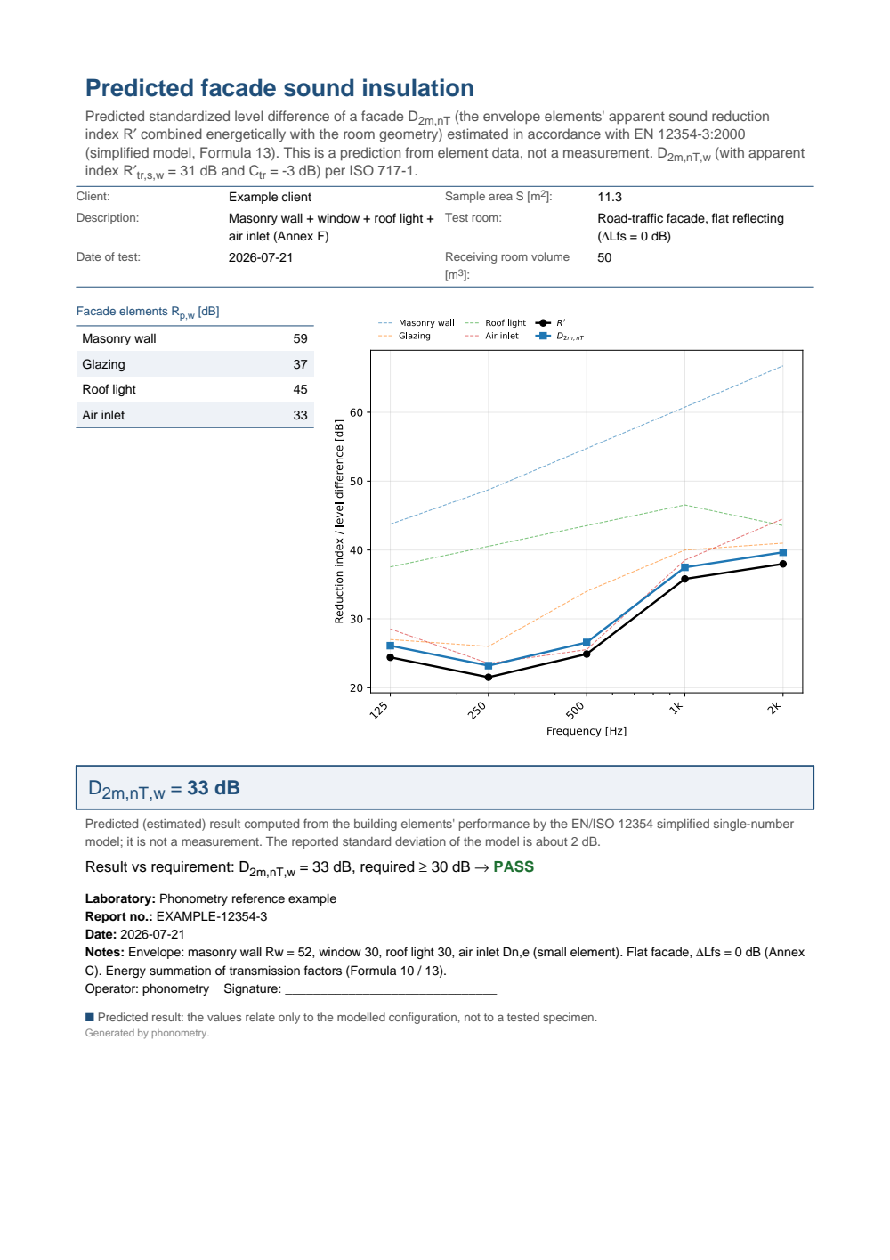
One-page predicted facade sound insulation report (EN 12354-3 Annex F): the metadata header (facade element set, exposed area, receiving-room volume, traffic situation), the facade-element table (each element's weighted partial index Rp,w) beside the per-element partial-index and R' / D2m,nT chart, the boxed predicted D2m,nT,w = 33 dB (with R'tr,s,w = 31 and Ctr = -3), the prediction statement noting the model's ~2 dB standard deviation and a PASS verdict against the 30 dB requirement.
Part 4: indoor → outdoor. The sound power level radiated by a segment (Formula 2) is with m² and the inside-field diffusivity term (Annex B; −6 dB ideal diffuse, −5 dB average industrial). Openings are elements whose “R” is the silencer insertion loss (a bare opening is 0 dB). The exterior level follows from the simplified Annex E attenuation of a finite radiating side, .
from phonometry import building
# EN 12354-4 Annex G, side 1: a 10×20 m concrete wall segment with a 6×4 m# industrial door, inside level Lp,in, Cd = -5 dB. The 40 dB cap on R' is an# Annex G example footnote (field leaks), not part of Formula (2)/(3): pass it# explicitly to reproduce Annex G; by default no cap is applied.bands = [63, 125, 250, 500, 1000, 2000, 4000, 8000]seg = building.radiated_sound_power(    [building.FacadeElement("wall", area=176.0, r=[32, 36, 36, 33, 39, 49, 57, 63]),     building.FacadeElement("door", area=24.0,  r=[21, 23, 28, 30, 30, 30, 30, 30])],    lp_in=[70, 74, 76, 72, 70, 67, 62, 57], area=200.0, c_d=-5.0,    r_prime_cap=40.0, octave_bands=bands)print(round(seg.l_w[0], 1), round(seg.l_w[1], 1))     # 59.8 61.2  (LW at 63/125 Hz)
# Exterior level 5 m in front of the centre of the 60×10 m side (LWA = 62.9 dB(A)).a_tot = building.outdoor_attenuation(width=60.0, height=10.0, distance=5.0)print(round(a_tot, 1), round(building.outdoor_level(62.9, a_tot), 1))   # 26.3 36.6
seg.plot()   # radiated LW per octave with the A-weighted LWA line (needs matplotlib)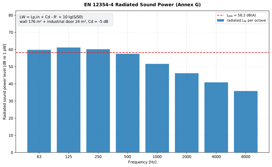
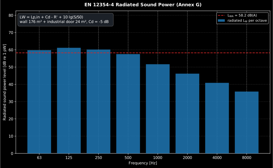
The Annex G side-1 segment: the wall dominates the area but the door’s weaker carries the radiated power, so the octave spectrum stays flat where the wall alone would fall. The dashed line is the A-weighted single number formed from the octave bands.
Show the code for this figure
import matplotlib.pyplot as pltimport numpy as npfrom phonometry import building
# EN 12354-4 Annex G, side 1: a 10×20 m concrete wall segment with a 6×4 m# industrial door, inside level Lp,in, Cd = -5 dB.bands = [63, 125, 250, 500, 1000, 2000, 4000, 8000]seg = building.radiated_sound_power(    [building.FacadeElement("wall", area=176.0, r=[32, 36, 36, 33, 39, 49, 57, 63]),     building.FacadeElement("door", area=24.0,  r=[21, 23, 28, 30, 30, 30, 30, 30])],    lp_in=[70, 74, 76, 72, 70, 67, 62, 57], area=200.0, c_d=-5.0,    r_prime_cap=40.0, octave_bands=bands)
# One line — LW per octave with the A-weighted LWA line:seg.plot()plt.show()
# By hand, from the result's fields:x = np.arange(len(bands))fig, ax = plt.subplots()ax.bar(x, seg.l_w, label="radiated LW per octave")ax.axhline(seg.l_w_dba, ls="--", color="tab:red",           label=f"LWA = {seg.l_w_dba:.1f} dB(A)")ax.set_xticks(x, [str(b) for b in bands])ax.set_xlabel("Frequency [Hz]")ax.set_ylabel("Radiated sound power level [dB re 1 pW]")ax.set_title("EN 12354-4 radiated sound power (Annex G)")ax.legend()plt.show()
Worked-example note. The 2000 worked examples carry small internal rounding inconsistencies at the higher octave bands (Part 3’s printed disagrees with its own per-element partial indices at 1 k/2 k; Part 4’s rows above 500 Hz disagree with its Table G.2 inputs). The implementation is faithful to the formulas: it reproduces the low bands, every single-number rating and the whole Annex E propagation exactly.
FacadeElement / facade_sound_reduction() / radiated_sound_power() parameters
Section titled “FacadeElement / facade_sound_reduction() / radiated_sound_power() parameters”| Parameter | Type | Units | Range / default | Notes |
|---|---|---|---|---|
FacadeElement.area | float | m² | > 0 for r / insertion_loss | Element area (ignored for dn_e) |
FacadeElement.r / dn_e / insertion_loss | float or seq | dB | give exactly one | Area element / small-element / opening insertion loss |
facade_sound_reduction(area) | float | m² | > 0 | Total façade area |
facade_sound_reduction(volume) | float | m³ | > 0 | Receiving-room volume (Formula 13) |
facade_sound_reduction(delta_l_fs) | float | dB | default 0 | Façade-shape term (Annex C; look it up with facade_shape_level_difference) |
radiated_sound_power(lp_in) | float or seq | dB | — | Inside level per band |
radiated_sound_power(c_d) | float | dB | default -6 | Diffusivity term (Annex B) |
radiated_sound_power(r_prime_cap) | float | dB | default None (off) | Optional field cap on , an Annex G example footnote (it uses 40 dB), not part of Formula (2)/(3) |
radiated_sound_power(octave_bands) | seq of int | Hz | default None | Octave centres matching the bands; enables the A-weighted |
facade_sound_reduction(frequencies) | seq | Hz | default None; length = band count | Band centres carried on the result for plotting |
outdoor_attenuation(width, height, distance) | float | m | > 0 | Finite radiating side and reception distance (Annex E) |
outdoor_level(l_w, attenuation) | float or seq | dB | broadcast-compatible | Exterior from one or more sides (Formula E.1) |
facade_sound_reduction() returns a FacadePredictionResult (r_prime, r_45,
r_tr_s, d_2m_nt, element_r, and the r_tr_s_w / d_2m_nt_w / c_tr single
numbers); radiated_sound_power() a RadiatedPowerResult (l_w, r_prime,
l_w_dba). Both expose .plot().
See also
Section titled “See also”- Field Insulation Measurement and Ratings: the measured in-situ quantities the prediction is checked against.
- Laboratory Insulation Measurement: the ISO 10140 ratings and ISO 10848 junction data the model consumes.
- Sound absorption in enclosed spaces (EN 12354-6): the absorption member of the same EN 12354 family.
- Dynamic stiffness of resilient materials (EN 29052-1): the s’ input to the EN 12354-2 floating-floor term.
- API reference:
building.building_predictionandbuilding.facade_prediction.
References
Section titled “References”- European Committee for Standardization. (2000). Building acoustics — Estimation of acoustic performance of buildings from the performance of elements — Part 1: Airborne sound insulation between rooms (EN 12354-1:2000). The simplified airborne flanking-transmission prediction (Annex E junctions, worked example H.3). The linked catalogue record is the BSI Knowledge page for BS EN 12354-1:2000.
- European Committee for Standardization. (2000). Building acoustics — Estimation of acoustic performance of buildings from the performance of elements — Part 2: Impact sound insulation between rooms (EN 12354-2:2000). The simplified impact flanking-transmission prediction (worked example E.3). The linked catalogue record is the BSI Knowledge page for BS EN 12354-2:2000.
- European Committee for Standardization. (2000). Building acoustics — Estimation of acoustic performance of buildings from the performance of elements — Part 3: Airborne sound insulation against outdoor sound (EN 12354-3:2000). The façade sound insulation prediction (Annex F worked example). The linked catalogue record is the BSI Knowledge page for BS EN 12354-3:2000.
- European Committee for Standardization. (2000). Building acoustics — Estimation of acoustic performance of buildings from the performance of elements — Part 4: Transmission of indoor sound to the outside (EN 12354-4:2000). The outdoor-radiation prediction (Annex G worked example). The linked catalogue record is the BSI Knowledge page for BS EN 12354-4:2000.
- Hopkins, C. (2007). Sound insulation. Butterworth-Heinemann. https://doi.org/10.4324/9780080550473The full treatment of flanking transmission and the EN 12354 prediction framework, from the vibration reduction index to its statistical basis. ISBN 978-0-7506-6526-1.