Mechanical mobility and the FRF family (ISO 7626-1)

Mechanical mobility is the complex ratio of a velocity response to the force that produces it, Y = v/F. It is one member of a family of motion-per-force frequency-response functions (FRFs): which one is used depends only on whether the motion is a displacement, a velocity or an acceleration, and each has a force-per-motion reciprocal. ISO 7626-1:2011 defines the whole family (Table 1, with the 3.1.2 mobility definition), and the classic closed-form single-degree-of-freedom (SDOF) resonator serves as the reference for those definitions. ISO 7626-2:2015 adds the measurement side: FRF estimation from measured signals and its acceptance criteria. This FRF backbone underpins the structure-borne source and transmission standards: ISO 9611, ISO 10846, EN 15657 and EN 12354-5.

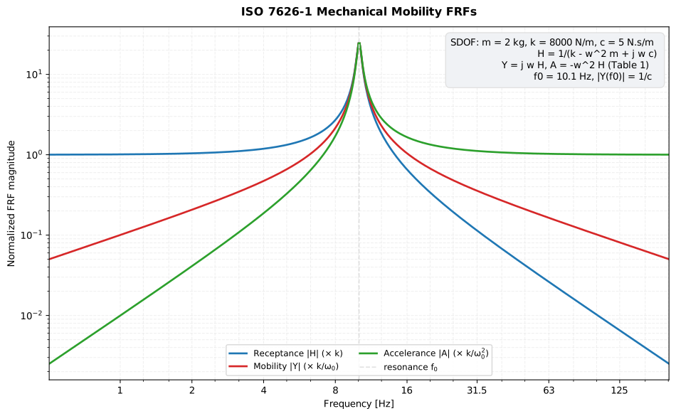
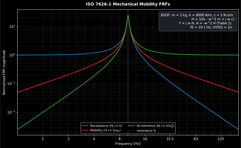
Show the code for this figure

import matplotlib.pyplot as plt
import numpy as np
from phonometry import vibration

m, k, c = 2.0, 8000.0, 5.0
f = np.logspace(np.log10(0.5), np.log10(200.0), 500)
w = 2.0 * np.pi * f
h = vibration.sdof_receptance(f, m, k, c)
for label, frf in (("receptance |H|", np.abs(h)),
                   ("mobility |Y|", np.abs(1j * w * h)),
                   ("accelerance |A|", np.abs(-(w**2) * h))):
    plt.loglog(f, frf / frf.max(), label=label)
plt.axvline(vibration.resonance_frequency(m, k), ls="--", color="0.6")
plt.xlabel("Frequency [Hz]"); plt.ylabel("Normalized magnitude")
plt.legend(); plt.show()

1. The frequency-response-function family (Table 1)

For a harmonic motion x·e^{jωt} the velocity is jω·x and the acceleration −ω²·x, so all three motion-per-force FRFs follow from the receptance H by a power of jω, and each has a force-per-motion reciprocal:

Motion	FRF (motion / force)	Unit	Reciprocal (force / motion)	Unit
displacement	receptance H = x/F	m/N	dynamic stiffness 1/H	N/m
velocity	mobility Y = jω·H	m/(N·s)	impedance 1/Y	N·s/m
acceleration	accelerance A = −ω²·H	1/kg	apparent mass 1/A	kg

convert_frf moves between any two of the six FRFs, pivoting through the receptance. A driving-point FRF has the response and force at the same point (i = j); a transfer FRF has them at different points. Note that the force-per-motion kinds are element-wise reciprocals: the free quantities of ISO 7626-1, 3.1.4; the blocked matrix quantities of Table 1 do not invert element-wise for multi-coordinate systems (Table 1 also names F/a the “effective mass”, the quantity called apparent mass here).

from phonometry import vibration

# A mobility of 2e-3 m/(N.s) at 80 Hz, expressed as the other FRFs:
Y = 2e-3
print(round(abs(vibration.convert_frf(Y, 80.0, "mobility", "impedance")), 1))     # 500.0  N.s/m
print(f"{abs(vibration.convert_frf(Y, 80.0, 'mobility', 'accelerance')):.3f}")    # 1.005  1/kg

The choice between the three motion FRFs is one of convenience, not physics: they carry the same information and convert_frf moves between them exactly. Accelerance is what an accelerometer-based measurement delivers directly; mobility is the natural currency of the structure-borne power standards (power is force times velocity, so P = ½·Re{Y}·|F|² at a contact); the reciprocals appear whenever a source is described by what it imposes rather than by how it responds. Reading a driving-point mobility plot is a structural diagnosis in itself: below a resonance the magnitude climbs proportionally to frequency along a stiffness line (|Y| ≈ ω/k), above it the magnitude falls along a mass line (|Y| ≈ 1/(ωm)), and the height of the peak between them reflects the damping: it equals 1/c for the isolated viscously damped resonator of the next section, while on real structures with overlapping modes damping is instead estimated by modal fitting or from the half-power bandwidth.

2. The SDOF reference resonator (closed form)

The canonical closed-form reference, expressed in the Table 1 / 3.1.2 FRF taxonomy, is a mass m, viscous damping c and stiffness k, whose receptance is

$$H(\omega )=\frac{1}{k-{\omega }^{2}m+j\omega c},{\omega }_0=\sqrt{k/m}.$$

At the resonance ω0 the driving-point mobility is purely real and equal to 1/c (the mobility peak measures the damping) while the static receptance (ω → 0) is the compliance 1/k:

import numpy as np
from phonometry import vibration

m, k, c = 2.0, 8000.0, 5.0
f0 = vibration.resonance_frequency(m, k)             # 10.07 Hz

y0 = complex(vibration.sdof_mobility(f0, m, k, c))
print(round(y0.real, 4), round(y0.imag, 6))   # 0.2 0.0   -> |Y(f0)| = 1/c
print(round(complex(vibration.sdof_receptance(1e-6, m, k, c)).real, 7))  # 0.000125 = 1/k

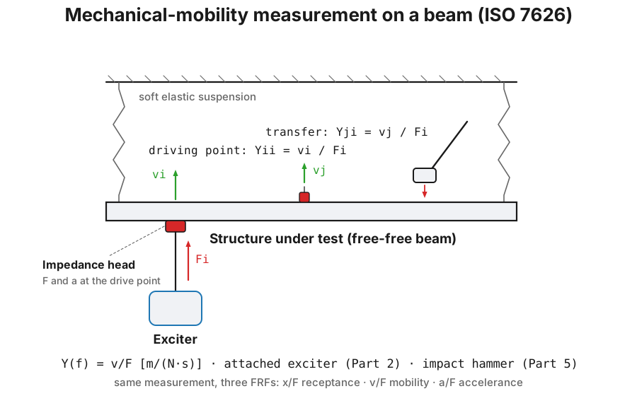
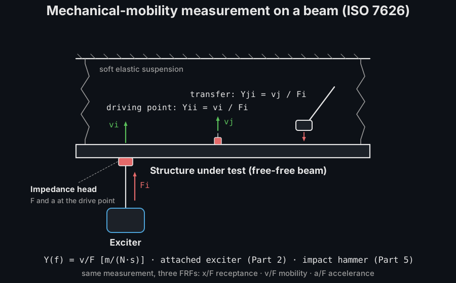
3. Measured FRFs and their acceptance criteria (ISO 7626-2)

In the usual ISO 7626-2 arrangement the structure hangs on a suspension soft enough that its rigid-body modes fall well below the first elastic resonance (the standard admits freely suspended or grounded structures; clause 5 asks for a support representative of the intended application), an exciter drives one point through an impedance head (a transducer stack measuring force and acceleration at the same point, which is what gives the attached-exciter setup its driving-point FRF), and accelerometers pick up the response elsewhere for the transfer FRFs. ISO 7626-5 covers the alternative of impact excitation with an exciter that is not attached to the structure, in practice usually an instrumented hammer: it trades the attached exciter’s controlled spectrum for speed, with an excitation spectrum set by the impactor mass and tip stiffness.

Processing measured random-excitation records per ISO 7626-2, 8.1.3 (the H1 estimator Ĥ = G(response, force)/G(force, force)) and the ordinary coherence γ² = |Gxy|²/(Gxx·Gyy) used for its data-quality checks are the library’s existing spectral estimators transfer_function and coherence (H1 is their default). On top of them, two ISO 7626-2 acceptance criteria are provided:

• Operational rigid-mass calibration (7.5.2). The measured FRF of a freely suspended rigid block of known mass must agree within ±5 % with |A| = 1/m (accelerance) or |Y| = 1/(2πf·m) (mobility).
• Random error (Annex A + 8.1.3). Enough spectra must be averaged that the normalized random error ε = √((1−γ²)/(2nγ²)) at each resonance of a driving-point mobility is below 5 %.

import numpy as np
from phonometry import vibration

# A 10 kg calibration block: |A| must be 1/m = 0.100 1/kg at every frequency.
f = np.array([20.0, 100.0, 500.0])
res = vibration.rigid_mass_calibration_check([0.100, 0.102, 0.097], f, mass=10.0)
print(res.passed, res.within_tolerance.tolist())   # True [True, True, True]

# The Annex A example: coherence 0.8 needs about 75 averages for < 5 %.
print(round(float(vibration.random_error_percent(0.8, 75)), 2))   # 4.08  %

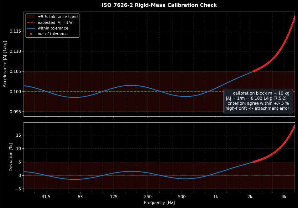
The calibration check returns a RigidMassCalibrationResult carrying the per-frequency deviation and pass flags, and a .plot(): the measured FRF magnitude against the rigid-mass line with its ±5 % tolerance band (upper panel) and the relative deviation against the same band (lower panel, where a few-percent tolerance is actually readable). A calibration that drifts out of the band towards a few kHz points at a transducer or attachment-compliance error, exactly what the check is meant to catch:

import numpy as np
from phonometry import vibration

m = 10.0                                                  # calibration block mass
f = np.logspace(np.log10(20.0), np.log10(5000.0), 400)
drift = 0.05 * (f / 2500.0) ** 2                          # high-frequency drift
measured = (1.0 / m) * (1.0 + 0.015 * np.sin(2 * np.pi * np.log10(f)) + drift)
res = vibration.rigid_mass_calibration_check(measured, f, mass=m)
print(res.passed)                                         # False (drift exceeds 5 %)
res.plot()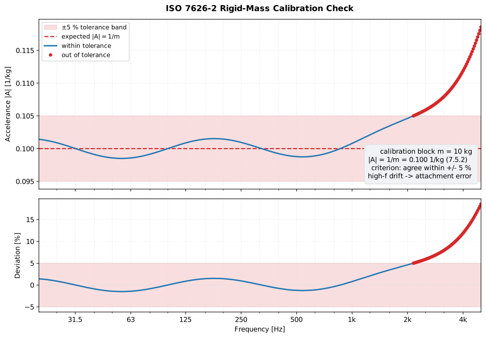

Show the code for this figure

import matplotlib.pyplot as plt
import numpy as np
from phonometry import vibration

m = 10.0
f = np.logspace(np.log10(20.0), np.log10(5000.0), 400)
drift = 0.05 * (f / 2500.0) ** 2
measured = (1.0 / m) * (1.0 + 0.015 * np.sin(2 * np.pi * np.log10(f)) + drift)
res = vibration.rigid_mass_calibration_check(measured, f, mass=m)
bad = ~res.within_tolerance

fig, (top, bot) = plt.subplots(2, 1, sharex=True, figsize=(10, 7),
                               gridspec_kw={"height_ratios": [1.5, 1.0]})
top.fill_between(f, res.expected * 0.95, res.expected * 1.05, color="C1",
                 alpha=0.15, label="±5 % tolerance band")
top.semilogx(f, res.expected, "--", color="C1", label="expected |A| = 1/m")
top.semilogx(f, res.measured, color="C0", label="within tolerance")
top.semilogx(f[bad], res.measured[bad], "o", color="C1", label="out of tolerance")
top.set_ylabel("Accelerance |A| [1/kg]"); top.legend()

bot.axhspan(-5.0, 5.0, color="C1", alpha=0.15)
bot.semilogx(f, 100.0 * res.deviation, color="C0")
bot.semilogx(f[bad], 100.0 * res.deviation[bad], "o", color="C1")
bot.set_xlabel("Frequency [Hz]"); bot.set_ylabel("Deviation [%]")
plt.show()

4. The MobilityResult bundle

sdof_mobility_result bundles the FRF over frequency into a MobilityResult, which exposes .magnitude, .phase, .to(target) (any Table-1 kind) and a .plot() of |Y(f)| with the resonance marked:

import numpy as np
from phonometry import vibration

f = np.logspace(np.log10(0.5), np.log10(200.0), 400)
res = vibration.sdof_mobility_result(f, mass=2.0, stiffness=8000.0, damping=5.0)
z = res.to("impedance")                        # impedance = 1/Y per frequency
print(res.frequencies[int(np.argmax(res.magnitude))].round(1))   # ~10.1 Hz

res.plot()   # |Y(f)| with the resonance marked (needs matplotlib)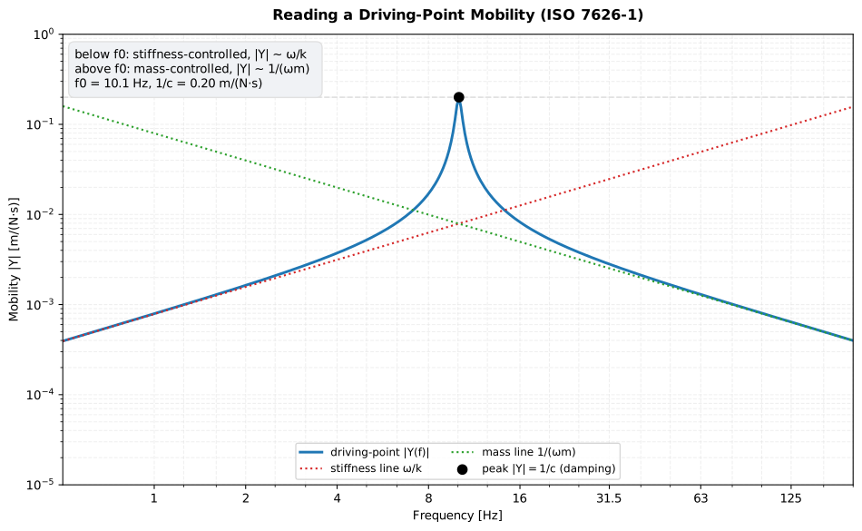

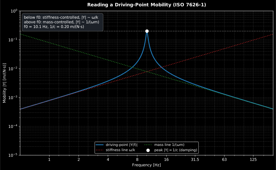
Reading a driving-point mobility is a structural diagnosis: below the resonance the magnitude climbs along the stiffness line $\omega /k$, above it it falls along the mass line $1/(\omega m)$, and the height of the peak between them is $1/c$, a direct read of the damping (Section 1).

Show the code for this figure

import matplotlib.pyplot as plt
import numpy as np
from phonometry import vibration

m, k, c = 2.0, 8000.0, 5.0
f = np.logspace(np.log10(0.5), np.log10(200.0), 400)
res = vibration.sdof_mobility_result(f, mass=m, stiffness=k, damping=c)

# One line — |Y(f)| with the resonance marked:
res.plot()
plt.show()

# By hand, adding the stiffness and mass asymptotes the prose describes:
w = 2.0 * np.pi * f
fig, ax = plt.subplots()
ax.loglog(f, res.magnitude, label="driving-point |Y(f)|")
ax.loglog(f, w / k, ":", label="stiffness line ω/k")
ax.loglog(f, 1.0 / (w * m), ":", label="mass line 1/(ωm)")
ax.axhline(1.0 / c, ls="--", color="0.6", label="peak |Y| = 1/c")
ax.set_xlabel("Frequency [Hz]")
ax.set_ylabel("Mobility |Y| [m/(N·s)]")
ax.set_title("Reading a driving-point mobility (ISO 7626-1)")
ax.legend()
plt.show()

Test-report fiche

MobilityResult.report(path) renders a one-page mechanical-mobility measurement report (ISO 7626-1:2011 FRF definitions, measurement per ISO 7626-2:2015). Mobility is a continuous frequency-response function, not an octave-band quantity, so the sheet presents it honestly as the $|Y(f)|$ magnitude spectrum plus a compact table of characteristic points (the FRF type, driving-point or transfer, the frequency range, the peak frequency, the peak mobility magnitude and the phase there), and a boxed peak mobility $|Y|$ at the frequency it occurs at (for a driving-point FRF a resonance, where $|Y|=1/c$ measures the damping). It is a characterisation, so there is no pass/fail verdict; language="es" renders the Spanish fiche. The fiche always embeds the $|Y(f)|$ spectrum, so it needs both the report and plot extras (pip install "phonometry[report,plot]").

from phonometry import ReportMetadata, vibration

res = vibration.sdof_mobility_result(f, mass=2.0, stiffness=8000.0, damping=5.0)
res.report(
    "mobility.pdf",
    metadata=ReportMetadata(
        specimen="Machine support bracket (driving point)",
        measurement_standard="ISO 7626-2",
    ),
)   # one-page fiche (needs phonometry[report,plot])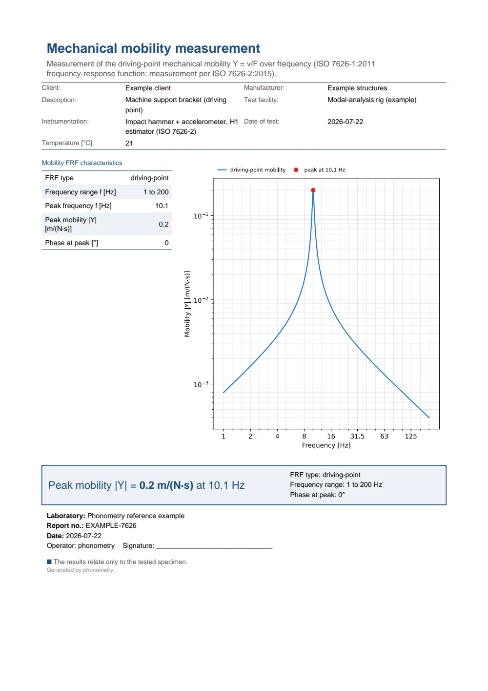

One-page mechanical-mobility fiche: a metadata header, a table of the FRF characteristic points (the FRF type, the frequency range, the peak frequency, the peak mobility magnitude and the phase there) beside the mobility magnitude spectrum, and the boxed peak mobility.

Download the report (PDF)

Mechanical-mobility fiche (MobilityResult.report): the FRF characteristic points and the mobility magnitude spectrum.

What this guide covers

Covered. ISO 7626-1:2011’s FRF family (Table 1): receptance, mobility and accelerance, with their force-per-motion reciprocals, moved between through convert_frf. Also covered are the driving-point/transfer distinction and the closed-form SDOF resonator used as their reference (sdof_receptance, sdof_mobility, sdof_accelerance, resonance_frequency, sdof_mobility_result). On the measurement side, ISO 7626-2:2015’s H1 processing of random excitation is covered too (transfer_function, coherence, shared with the electroacoustics guide), along with two acceptance criteria: the 7.5.2 rigid-mass operational calibration (rigid_mass_calibration_check) and the Annex A random-error criterion (random_error_percent).

Not covered. ISO 7626-5 covers impact-hammer excitation as an alternative to the attached exciter. It is named here for context only: no function synthesizes or processes an impact-excitation spectrum. The blocked matrix quantities of Table 1, needed for multi-coordinate systems, are not built either. convert_frf returns only the element-wise free reciprocals of ISO 7626-1, 3.1.4, correct for driving-point or single-path use but not for a full FRF matrix.

See also

• API reference: vibration.mechanical_mobility.

References

• Cremer, L., Heckl, M., & Petersson, B. A. T. (2005). Structure-borne sound: Structural vibrations and sound radiation at audio frequencies (3rd ed.). Springer. https://doi.org/10.1007/b137728The standard monograph on structural vibration: point and transfer mobilities of beams and plates, and the power flow P = ½·Re{Y}·|F|² that makes mobility the working quantity of this page. ISBN 978-3-540-22696-3.
• International Organization for Standardization. (2011). Mechanical vibration and shock — Experimental determination of mechanical mobility — Part 1: Basic terms and definitions, and transducer specifications (ISO 7626-1:2011). The FRF family and its reciprocals (Table 1, the 3.1.2 mobility and 3.1.4 free-quantity definitions), the free/blocked distinctions and the driving-point / transfer distinction implemented here. Conformance is anchored on the closed-form SDOF identities consistent with those definitions: the driving-point mobility peak |Y(ω0)| = 1/c, the static receptance H(0) = 1/k and the exact Table-1 reciprocity impedance·mobility = 1.
• International Organization for Standardization. (2015). Mechanical vibration and shock — Experimental determination of mechanical mobility — Part 2: Measurements using single-point translation excitation with an attached vibration exciter (ISO 7626-2:2015). The measurement side: the 8.1.3 H1 processing of random excitation, the 7.5.2 rigid-mass operational calibration (±5 %) and the Annex A random-error criterion (< 5 % at resonances). Conformance is anchored on the rigid-mass calibration values (|A| = 0.100 1/kg for 10 kg; |Y| = 1.59155e-4 m/(N·s) at 100 Hz) and the Annex A example (γ² = 0.8, n = 75 → ε = 4.08 %).