Industrial Noise Control: Silencers, HVAC and Enclosures

Three passive measures dominate applied noise control: silencers in a duct, the passive attenuations and regenerated noise of an HVAC run, and a machine enclosure. phonometry.noise_control covers all three with the engineering theory of Bies, Hansen & Howard. The silencers are built on the one-dimensional four-pole (transfer-matrix) method, which chains reusable acoustic elements; the HVAC methods are the ASHRAE tables and closed forms for bends, end reflection, plenums and flow noise; and the enclosure model combines a user-supplied panel transmission loss with the reverberant build-up inside the enclosure. The radiating piston of the electroacoustics domain is the companion radiator model.

1. Reactive silencers (four-pole method)

A reactive silencer attenuates by reflecting sound with impedance discontinuities. Each acoustic element is a 2x2 transfer matrix relating the pressure p and volume velocity Su at its two ends, and a compound silencer is the ordered matrix product of its elements (Bies §8.9). A straight duct of length L and area S is

$$\left[\begin{array}{cc}\cos kL& j\frac{\rho c}{S}\sin kL\\ j\frac{S}{\rho c}\sin kL& \cos kL\end{array}\right],k=\omega /c,$$

and a side branch of impedance $Z_b$ is the shunt $\left[\begin{array}{cc}1& 0\\ 1/Z_b& 1\end{array}\right]$. The transmission loss follows from the compound matrix $T$ with the port impedances $Z_1=\rho c/S_{\text{in}}$ and $Z_n=\rho c/S_{\text{out}}$ (Munjal Eq. (3.27); Bies Eq. (8.141) prints the $T_{11}$/$T_{22}$ impedance weights of this formula inverted and fails the sudden-expansion limit, see the errata registry)

$$\mathrm{TL}=10{\log }_{10}\left[\frac{Z_n}{Z_1}\frac{1}{4}{\left|T_{11}+\frac{T_{12}}{Z_n}+Z_1{T}_{21}+\frac{Z_1}{Z_n}{T}_{22}\right|}^2\right],$$

which for equal inlet/outlet areas $S$ reduces to (Bies Eq. (8.148))

$$\mathrm{TL}=20{\log }_{10}\left(\frac{1}{2}\left|T_{11}+\frac{T_{12}}{Z_c}+Z_c{T}_{21}+T_{22}\right|\right),Z_c=\frac{\rho c}{S},$$

and the insertion loss for a source impedance $Z_s$ and radiation impedance $Z_r$ is the extra attenuation over a direct connection.

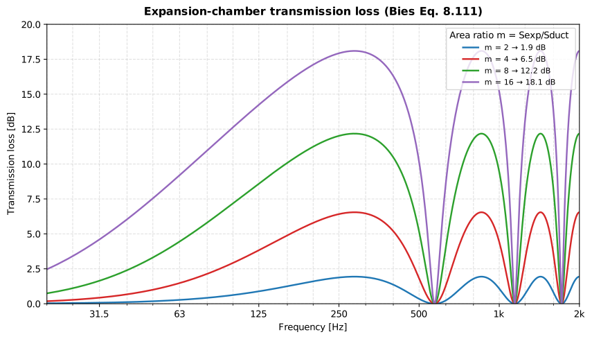
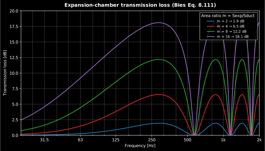
Expansion chamber

The simplest silencer, a chamber of area $S_{\text{exp}}$ and length $L$ between pipes of area $S_{\text{duct}}$, has the closed-form transmission loss (Bies Eq. (8.111)) with area ratio $m=S_{\text{exp}}/S_{\text{duct}}$

$$\mathrm{TL}=10{\log }_{10}\left[1+\frac{1}{4}{\left(m-\frac{1}{m}\right)}^2{\sin }^{2}kL\right],$$

peaking at $10{\log }_{10}[1+\frac{1}{4}(m-1/m{)}^2]$ when $kL=\pi /2,3\pi /2,\dots$ and dropping to $0$ at $kL=n\pi$ where the chamber is a half-wavelength long and transparent. The four-pole product reproduces this exactly.

import numpy as np
from phonometry import expansion_chamber

freqs = np.linspace(20.0, 2000.0, 2000)
res = expansion_chamber(freqs, length=0.3, chamber_area=0.04, pipe_area=0.01)
print(round(res.transmission_loss.max(), 2))   # 6.55 dB peak (m = 4)
# The troughs at f = n c / 2L are exactly 0 dB (no dissipation).
print(round(float(res.transmission_loss[np.argmin(res.transmission_loss)]), 6))

The one-liner res.plot() draws the transmission loss of the chamber (and its insertion loss when the source and radiation impedances are given). The figure below sweeps the area ratio instead: a larger mismatch $m$ lifts every peak, but the troughs stay at 0 dB and the peaks stay at the same frequencies, set only by the chamber length.

Show the code for this figure

import matplotlib.pyplot as plt
import numpy as np
from phonometry import expansion_chamber

freqs = np.linspace(20.0, 2000.0, 2000)

# One line for one chamber: TL vs frequency (with the insertion loss too if
# source/radiation impedances are given).
expansion_chamber(freqs, 0.3, 0.04, 0.01,
                  source_impedance=4e4, radiation_impedance=5e3).plot()
plt.show()

# By hand: the family of area ratios of the concept figure.
fig, ax = plt.subplots()
for m in (2.0, 4.0, 8.0, 16.0):
    res = expansion_chamber(freqs, 0.3, m * 0.01, 0.01)
    ax.plot(freqs, res.transmission_loss, label=f"m = {int(m)}")
ax.set_xlabel("Frequency [Hz]"); ax.set_ylabel("Transmission loss [dB]")
ax.legend()
plt.show()

Side-branch and extended-tube resonators

A Helmholtz resonator (neck area $S_n$, effective length $l_e$, cavity volume $V$) and a closed quarter-wave tube (length $l_e$) each short the duct at their tuning frequency, giving a sharp transmission-loss spike there: $f_0=\frac{c}{2\pi }\sqrt{S_n/(l_{e}V)}$ (Bies Eq. (8.46)) and $f=c/4l_e$ (Eq. (8.44)). An extended-tube chamber buries quarter-wave side branches in an expansion chamber to fill the plain chamber’s troughs.

import numpy as np
from phonometry import (
    helmholtz_resonator, quarter_wave_resonator, extended_tube_chamber,
)

f = np.linspace(20.0, 600.0, 4000)

hr = helmholtz_resonator(f, duct_area=0.01, neck_area=1e-4,
                         neck_length=0.02, cavity_volume=1e-3)
print(round(float(hr.resonances[0]), 1))       # tuning frequency, Hz
hr.plot()   # TL spike at the tuning frequency (needs matplotlib)

qw = quarter_wave_resonator(f, duct_area=0.01, length=1.516, branch_area=2e-3,
                            speed_of_sound=343.24)
print(round(float(qw.resonances[0]), 1))        # 56.6 Hz (Bies Example 8.1)

# An inlet extension of L/4 fills the first expansion-chamber trough.
et = extended_tube_chamber(f, length=0.4, chamber_area=0.04, pipe_area=0.01,
                           inlet_extension=0.1)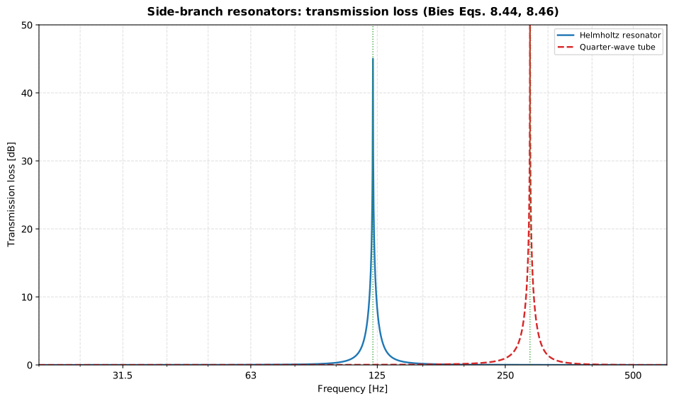

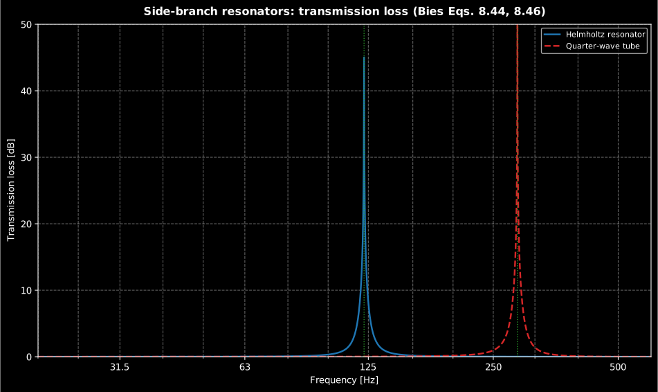
Each side branch shorts the duct at its own tuning frequency and is nearly transparent elsewhere: the narrow spike is why resonators are matched to a firing frequency or a fan blade-passing tone rather than used broadband.

Show the code for this figure

import matplotlib.pyplot as plt
import numpy as np
from phonometry import helmholtz_resonator, quarter_wave_resonator

f = np.linspace(20.0, 600.0, 4000)
hr = helmholtz_resonator(f, duct_area=0.01, neck_area=1e-4,
                         neck_length=0.02, cavity_volume=1e-3)
qw = quarter_wave_resonator(f, duct_area=0.01, length=0.3, branch_area=2e-3)

# One line for one device: TL vs frequency with the resonance marked.
hr.plot()
plt.show()

# By hand: both side branches on the same axes.
fig, ax = plt.subplots()
ax.plot(f, hr.transmission_loss, label="Helmholtz resonator")
ax.plot(f, qw.transmission_loss, "--", label="Quarter-wave tube")
for fr in (hr.resonances[0], qw.resonances[0]):
    ax.axvline(float(fr), ls=":", color="#2ca02c")
ax.set_xlabel("Frequency [Hz]"); ax.set_ylabel("Transmission loss [dB]")
ax.set_ylim(0.0, 50.0)
ax.legend()
plt.show()

Each returns a ReactiveSilencerResult with transmission_loss, insertion_loss (when impedances are given), the compound transfer_matrix and .plot(). Advanced layouts chain elements directly with duct_matrix, shunt_matrix, cascade, transmission_loss and insertion_loss.

2. HVAC duct attenuation and flow noise

A ventilation run attenuates fan noise at bends, at the open duct end and in plenums, and regenerates noise wherever the airflow is disturbed. phonometry.noise_control.hvac gathers the Bies Chapter 8 methods.

from phonometry.noise_control import hvac

bands = [63.0, 125.0, 250.0, 500.0, 1000.0, 2000.0]

# Low-frequency reflection back up an open duct end (ASHRAE Table 8.14).
er = hvac.end_reflection_loss(bands, diameter=0.30, termination="flush")

# Insertion loss of a lined square 90-degree elbow (ASHRAE Table 8.11).
el = hvac.elbow_insertion_loss(bands, width=0.3, bend_type="square", lined=True)
er.plot()   # the band attenuation (or regenerated Lw) in one line (needs matplotlib)

# Plenum-chamber TL by Wells' method (closed form).
tl = hvac.plenum_attenuation(exit_area=0.1, line_of_sight=1.0,
                             wall_area=20.0, mean_absorption=0.2)
print(round(tl, 1))                              # dB

# Flow-generated (self) noise of a straight duct (VDI 2081).
fn = hvac.flow_noise_straight_duct(bands, flow_velocity=10.0, area=0.04)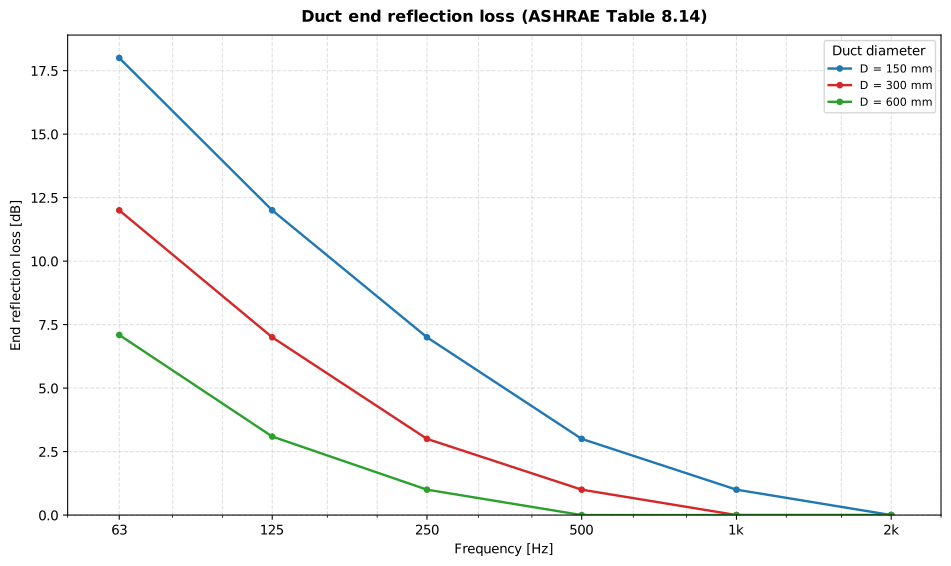

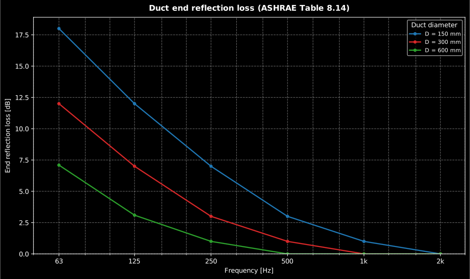
The open end of a duct reflects low-frequency energy back up the run — for free, before any silencer: the smaller the duct against the wavelength, the larger the loss, which is why small diffuser necks tame low-frequency fan rumble and why the correction must not be double-counted when a manufacturer’s diffuser data already includes it.

Show the code for this figure

import matplotlib.pyplot as plt
import numpy as np
from phonometry.noise_control import hvac

bands = [63.0, 125.0, 250.0, 500.0, 1000.0, 2000.0]

# One line for one duct: the HvacSpectrumResult of the 300 mm flush end.
er = hvac.end_reflection_loss(bands, diameter=0.30, termination="flush")
er.plot()
plt.show()

# By hand: the family over duct diameters of the concept figure.
fig, ax = plt.subplots()
for diameter in (0.15, 0.30, 0.60):
    er = hvac.end_reflection_loss(bands, diameter=diameter, termination="flush")
    ax.semilogx(er.frequencies, er.values, "o-",
                label=f"D = {int(diameter * 1000)} mm")
ax.set_xlabel("Frequency [Hz]"); ax.set_ylabel("End reflection loss [dB]")
ax.legend(title="Duct diameter")
plt.show()

The end-reflection and elbow methods interpolate the ASHRAE tables (they pass exactly through the tabulated nodes); the plenum (Wells) and flow-noise (VDI 2081) methods are closed forms. end_reflection_loss, elbow_insertion_loss, flow_noise_straight_duct and flow_noise_bend return an HvacSpectrumResult (attenuation or regenerated sound power level) with .plot(); plenum_attenuation returns the transmission loss directly. Rectangular ducts use the equivalent diameter $D=\sqrt{4S/\pi }$.

Note

Bies 5th ed. gives the duct end reflection only as the ASHRAE Table 8.14 look-up; there is no closed form in that edition. This module reproduces and interpolates the table.

3. Machine enclosures

A sealed enclosure reduces the radiated noise by its panel transmission loss $R$, minus a penalty $C$ for the reverberant build-up inside the small, hard cavity (Bies Eqs. (7.103), (7.111)):

$$\mathrm{IL}=R-C,C=10{\log }_{10}\left(0.3+\frac{S_E}{R_i}\right),$$

with the external area $S_E$ and the interior room constant $R_i=S_i{\alpha }_i/(1-{\alpha }_i)$ (the same room_constant as the steady-state room field). A hard interior wastes much of the panel $R$; lining it drives $C$ toward its floor $10{\log }_{10}0.3=-5.2$ dB.

The panel transmission loss $R$ is supplied by you as a per-band array (measured, or predicted by a panel model), or as a callable of frequency. This module never predicts $R$ itself; it combines a given $R$ with the interior absorption.

import numpy as np
from phonometry import enclosure_insertion_loss

bands = np.array([125.0, 250.0, 500.0, 1000.0, 2000.0, 4000.0])
panel_R = np.array([18.0, 24.0, 30.0, 36.0, 42.0, 46.0])   # measured, dB

enc = enclosure_insertion_loss(
    panel_R, external_area=6.0, internal_area=5.0,
    internal_absorption=0.3, frequencies=bands,
)
print(np.round(enc.insertion_loss, 1))            # net IL = R - C per band
enc.plot()                                         # panel R, correction C and IL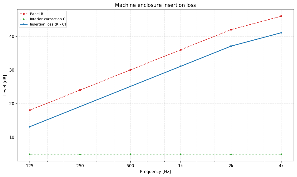

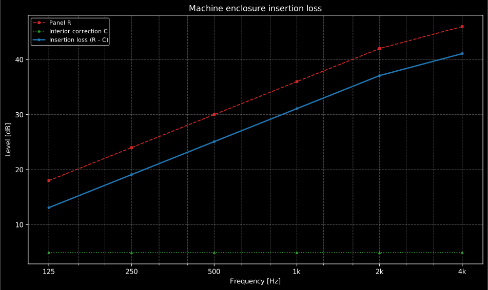
What the enclosure delivers is R − C, not the panel R: even this lined interior (mean absorption 0.3) costs about 5 dB of the panel’s rating in every band, and a hard, unlined interior would cost far more. Budget the lining together with the panels, not as an afterthought.

Show the code for this figure

import matplotlib.pyplot as plt
import numpy as np
from phonometry import enclosure_insertion_loss

bands = np.array([125.0, 250.0, 500.0, 1000.0, 2000.0, 4000.0])
panel_R = np.array([18.0, 24.0, 30.0, 36.0, 42.0, 46.0])   # measured, dB

enc = enclosure_insertion_loss(
    panel_R, external_area=6.0, internal_area=5.0,
    internal_absorption=0.3, frequencies=bands,
)

# One line — panel R, interior correction C and the net IL = R - C:
enc.plot()
plt.show()

# By hand, from the per-band fields the result carries:
fig, ax = plt.subplots()
ax.plot(bands, enc.panel_transmission_loss, "s--", label="Panel R")
ax.plot(bands, enc.correction, "^:", label="Interior correction C")
ax.plot(bands, enc.insertion_loss, "o-", label="Insertion loss (R - C)")
ax.set_xlabel("Frequency [Hz]"); ax.set_ylabel("Level [dB]")
ax.set_xscale("log")
ax.legend()
plt.show()

enclosure_insertion_loss returns an EnclosureResult with the panel panel_transmission_loss, the interior correction, the net insertion_loss, the interior room_constant, and .plot().

Cross-check against the FDTD solver

The four-pole expansion chamber is cross-checked against the independent 2D FDTD wave solver: a plane-wave duct that widens into a chamber and narrows back transmits far less at the four-pole TL peak ($kL=\pi /2$) than at the transparent trough ($kL=\pi$), and the measured amplitude ratio reproduces the closed-form peak transmission loss to a fraction of a decibel.

What this guide covers

Covered. Reactive silencers by the four-pole transfer-matrix method (Bies §8.8-8.9, Munjal Eq. (3.27)): the closed-form expansion_chamber (Eq. (8.111)), helmholtz_resonator and quarter_wave_resonator (Eqs. (8.46), (8.44)), extended_tube_chamber, and the duct_matrix/ shunt_matrix/cascade building blocks, cross-checked against the independent FDTD solver. The Bies §8.11-8.17 / ASHRAE HVAC methods: hvac.end_reflection_loss and hvac.elbow_insertion_loss (interpolated tables), hvac.plenum_attenuation (Wells closed form) and hvac.flow_noise_straight_duct/flow_noise_bend (VDI 2081). The machine- enclosure insertion loss of Bies §7.4 (Eqs. (7.103), (7.111)), enclosure_insertion_loss, combining a supplied panel transmission loss with the interior room-constant correction.

Not covered. Only reactive elements are implemented: dissipative (absorptive, duct-lining) silencers are not modelled. enclosure_insertion_loss never predicts the panel transmission loss R itself; you supply it measured or from another model, and the module only combines it with the interior correction.

See also

• Electroacoustics: the radiating piston (radiation impedance and directivity), the companion radiator model.
• Sound Power: the source Lw that feeds a duct or an enclosure.
• Room image sources and steady field: the room_constant reused by the enclosure interior correction.
• 2D FDTD wave simulation: the independent solver that cross-checks the expansion chamber.
• Conformance report: the closed forms and worked anchors these implementations are validated against.
• API reference: noise_control.silencers, noise_control.hvac and noise_control.enclosures.

References

• Bies, D. A., Hansen, C. H., & Howard, C. Q. (2017). Engineering noise control (5th ed.). CRC Press. https://doi.org/10.1201/9781351228152The muffler four-pole method and expansion-chamber TL (§8.8-8.9), the HVAC duct methods (§8.11-8.17) and the machine-enclosure noise reduction (§7.4) of this page.
• Munjal, M. L. (2014). Acoustics of ducts and mufflers (2nd ed.). Wiley. https://doi.org/10.1002/9781118443767The transfer-matrix formulation, the element matrices and the transmission loss from the compound matrix (Eq. (3.27)) behind §1.
• Vér, I. L., & Beranek, L. L. (2006). Noise and vibration control engineering: Principles and applications (2nd ed.). Wiley. https://doi.org/10.1002/9780470172568The companion treatment of mufflers, ducts and enclosures cross-checked in this page.