Getting Started

phonometry is a Python toolkit for acoustic measurement, from fractional octave filter banks and frequency weighting to sound levels and standardized metrics. Every metric is verified against its governing standard, 427 numerical checks in all. Install it with pip install phonometry; the first example below filters a signal into one-third octave bands and returns the sound pressure level of each band.

Installation

Option 1: From PyPI (Recommended)

pip install phonometry

Optional extras:

pip install phonometry[plot]    # matplotlib, for filter response plots and result .plot() methods
pip install phonometry[perf]    # numba, faster 'impulse' time weighting
pip install phonometry[report]  # reportlab + svglib, so result .report() methods render normative PDF fiches
pip install phonometry[full]    # all of the above

Option 2: Cloning and Installing

git clone https://github.com/jmrplens/phonometry.git
cd phonometry
pip install .

Option 3: Git Submodule

git submodule add https://github.com/jmrplens/phonometry.git
# Then install in editable mode to use it from your project
pip install -e ./phonometry

The processing chain at a glance

Every phonometry analysis is some subset of one pipeline: take the raw signal, convert it to physical units, weight it in frequency, split it into standardized bands, smooth it in time and reduce it to metrics:

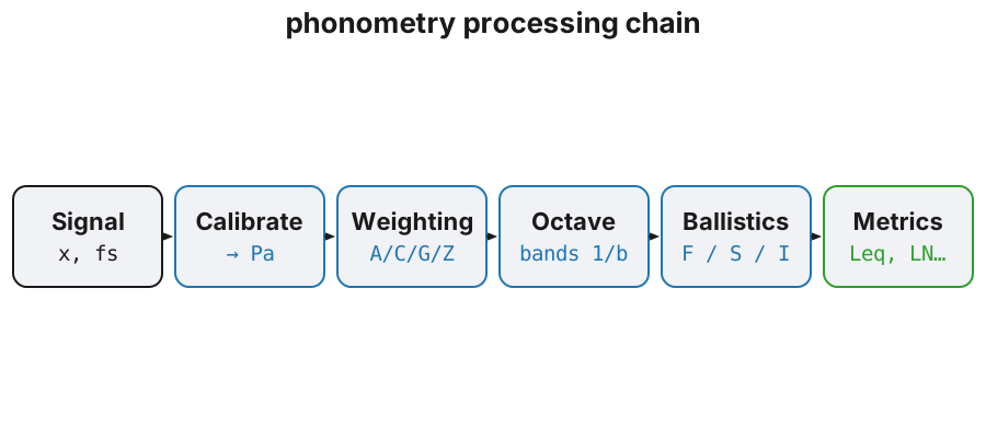
Each stage is an independent function or class you can use on its own; the guides cover them left to right (Calibration → Frequency Weighting → Filter Banks → Time Weighting → Levels).

Basic Usage: 1/3 Octave Analysis

Analyze a signal and get the Sound Pressure Level (SPL) per frequency band.

import numpy as np
from phonometry import metrology

fs = 48000
t = np.linspace(0, 1, fs, endpoint=False)
# Composite signal: 100Hz + 1000Hz
signal = np.sin(2 * np.pi * 100 * t) + np.sin(2 * np.pi * 1000 * t)

# Apply 1/3 octave filter bank
spl, freq = metrology.octave_filter(signal, fs=fs, fraction=3)

print(f"Bands: {freq}")
# Bands: [12.589254117941678, 15.848931924611138, ..., 19952.623149688785]  (33 bands)
print(f"SPL [dB]: {spl}")
# SPL [dB]: [46.88395351 47.96774897 49.04991279 ...]  — ~90.7 dB at 100 Hz and ~90.9 dB at 1 kHz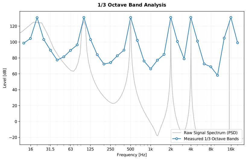

Example of a 1/3 Octave Band spectrum analysis of a complex signal.

Show the code for this figure

import matplotlib.pyplot as plt
import scipy.signal
import numpy as np
from phonometry import metrology

fs = 48000
t = np.linspace(0, 1, fs, endpoint=False)
# Composite signal: 100Hz + 1000Hz
signal = np.sin(2 * np.pi * 100 * t) + np.sin(2 * np.pi * 1000 * t)
# Apply 1/3 octave filter bank
spl, freq = metrology.octave_filter(signal, fs=fs, fraction=3)

# Gray background: the raw-signal PSD (Welch), shifted to sit just below the
# band SPLs so both spectral shapes share one axis.
f_psd, psd = scipy.signal.welch(signal, fs, nperseg=8192)
psd_db = 10 * np.log10(psd + 1e-12)
psd_db += np.max(spl) - np.max(psd_db) - 5

fig, ax = plt.subplots()
ax.semilogx(f_psd, psd_db, color="gray", alpha=0.6, label="Raw signal PSD")
ax.semilogx(freq, spl, marker="o", markerfacecolor="white",
            label="1/3 octave bands")
ax.set_xlabel("Frequency [Hz]")
ax.set_ylabel("SPL [dB]")
ax.legend()
plt.show()

Analyzing an audio file

from scipy.io import wavfile
from phonometry import metrology

# Load standard WAV file
fs, signal = wavfile.read("measurement.wav")

# Analyze
# Note: To obtain real-world SPL values, you must calibrate the input.
# See the Calibration guide.
spl, freq = metrology.octave_filter(signal, fs=fs, fraction=3)

Integer audio (e.g. int16 WAV data) is converted to float64 internally, so it is safe to pass wavfile.read output directly.

Where to go next

The octave analysis above uses the metrology core, one of fifteen domain namespaces; the sidebar sections walk through the rest, from psychoacoustics and room, building and vibration acoustics to environmental, aircraft and underwater noise, electroacoustics and FDTD wave simulation. Every result object exposes a one-line .plot(language="en"|"es") figure and, where a standard defines a reporting format, a .report() method that renders the normative PDF fiche.

• Filter Banks: choose an architecture and inspect responses
• Calibration and dBFS: get real-world SPL values
• Why phonometry: the conformance-first design philosophy
• Conformance report: the expected and computed value of all 427 checks
• API Reference: every parameter of every function
• Bibliography: the books and papers behind every guide, each with a verified link