Calibration and dBFS

Every level this library reports is only as trustworthy as the one number this page produces: the sensitivity factor that converts digital units into pascals. The page covers both reference frames a recording can be analyzed in: physical dB SPL, obtained by calibrating the chain against an IEC 60942 acoustic calibrator, and digital dBFS, levels relative to full scale with no physical claim attached.

Choosing between them is a question about your measurement chain, not about preference. Work in dB SPL whenever the result faces a physical criterion (a noise limit, an exposure threshold, any acoustics standard); that requires a calibrator recording made through the same, untouched chain as the measurement. Work in dBFS when the signal never had a calibrated analog front end (loudness normalization, codec and interface tests, file-only analysis) or when no calibration tone exists, in which case absolute SPL statements are simply out of reach.

The workflow around the factor matters as much as the formula: derive it before and re-check it after each session, verify meter and calibrator periodically in the laboratory (IEC 61672-3 and IEC 60942; Bies, Hansen & Howard 2017, §3.4), and treat the pre/post difference as your drift bound. The field, laboratory and drift section below turns that into concrete rules, and the Build a sound level meter walkthrough starts from exactly this step before any level is computed.

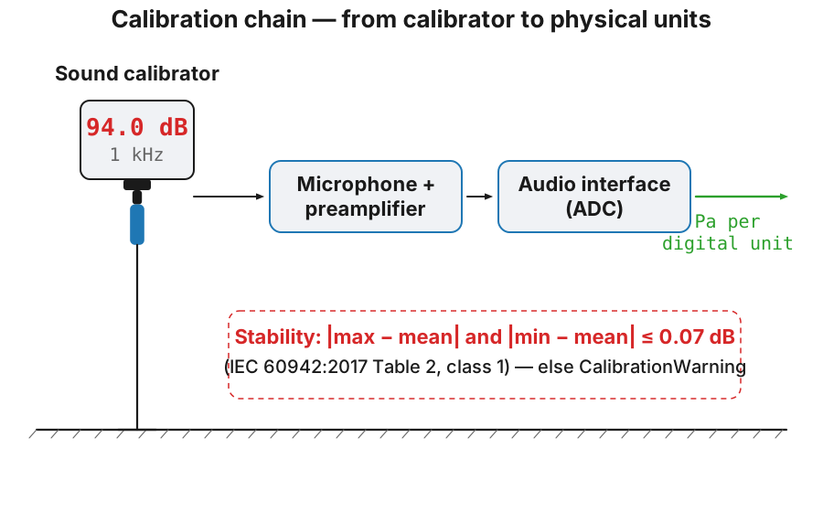
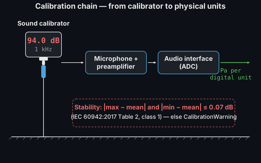
Why calibrate? The theory

A digital recording only knows numbers: a full-scale sine wave is ±1.0 regardless of whether it was a whisper or a jet engine. To report physical sound pressure levels the chain microphone → preamplifier → ADC must be characterized by a single number, the sensitivity factor $S$, that converts digital units into pascals:

$$p(t)=Sx(t)S=\frac{p_{\text{ref}}\cdot 10^{L_{\text{cal}}/20}}{{\tilde{x}}_{\text{ref}}}$$

where $L_{\text{cal}}$ is the calibrator’s level (typically 94 dB, i.e. 1 Pa), $p_{\text{ref}}=20\mu \text{Pa}$ and ${\tilde{x}}_{\text{ref}}$ is the RMS of the recorded calibration tone in digital units. sensitivity() is exactly that equation. The factor is valid as long as nothing in the chain changes: touch the gain knob and you must recalibrate.

Physical Calibration (Sound Level Meter)

To get accurate SPL measurements from a digital recording, you must first calculate the sensitivity of your measurement chain using a reference tone (e.g., 94 dB @ 1 kHz).

flowchart LR
    A["Calibrator tone\n94 dB @ 1 kHz\n(IEC 60942)"] --> B["Recording\ncalibrator_recording"]
    B --> C["sensitivity()"]
    C --> D["calibration_factor\n(digital units → Pa)"]
    D --> E["octave_filter / leq / laeq / ln_levels"]
    F["Measurement\nrecording"] --> E
    E --> G["Levels in dB SPL\n(re 20 µPa)"]

import numpy as np
from phonometry import metrology

# 1. Record your 94 dB calibrator signal (1 kHz, 1 Pa RMS = 94 dB SPL)
fs = 48000
# calibrator_recording: your recorded 1 kHz calibrator tone (1 Pa RMS = 94 dB SPL).
#   Synthesized here so the guide runs; in a real measurement, record your calibrator.
calibrator_recording = np.sqrt(2) * np.sin(2 * np.pi * 1000 * np.arange(fs) / fs)
# recording: the mic capture you want to calibrate, same input chain (Pa after calibration).
#   Synthesized here; in a real measurement this is your recorded signal.
recording = 0.2 * np.sin(2 * np.pi * 1000 * np.arange(fs) / fs)

# 2. Calculate the sensitivity factor
calibration_factor = metrology.sensitivity(calibrator_recording, target_spl=94.0, fs=fs)

# 3. Apply calibration to your measurements
spl, freq = metrology.octave_filter(recording, fs, calibration_factor=calibration_factor)
# Now 'spl' values are in real-world dB SPL!

The same calibration_factor works across the whole library: octave_filter, OctaveFilterBank, leq, laeq and ln_levels.

Calibrator assumptions (IEC 60942)

sensitivity assumes the reference recording comes from an acoustic calibrator as specified by IEC 60942 (classes LS, 1 and 2):

• The default target_spl=94.0 matches the common 94 dB @ 1 kHz calibrator output (the standard requires the principal level to be at least 90 dB re 20 µPa; 94 dB and 114 dB are the usual choices).
• The resulting sensitivity inherits the calibrator’s class tolerance (e.g. ±0.4 dB for a class 1 calibrator between 160 Hz and 1.25 kHz, IEC 60942 Table 1) plus the RMS estimation error of your recording.
• IEC 60942 specifies the generated level as a 20 s average: record a few seconds of stable tone (excluding handling noise at the start/end) for the RMS estimate to converge.

Automatic stability validation

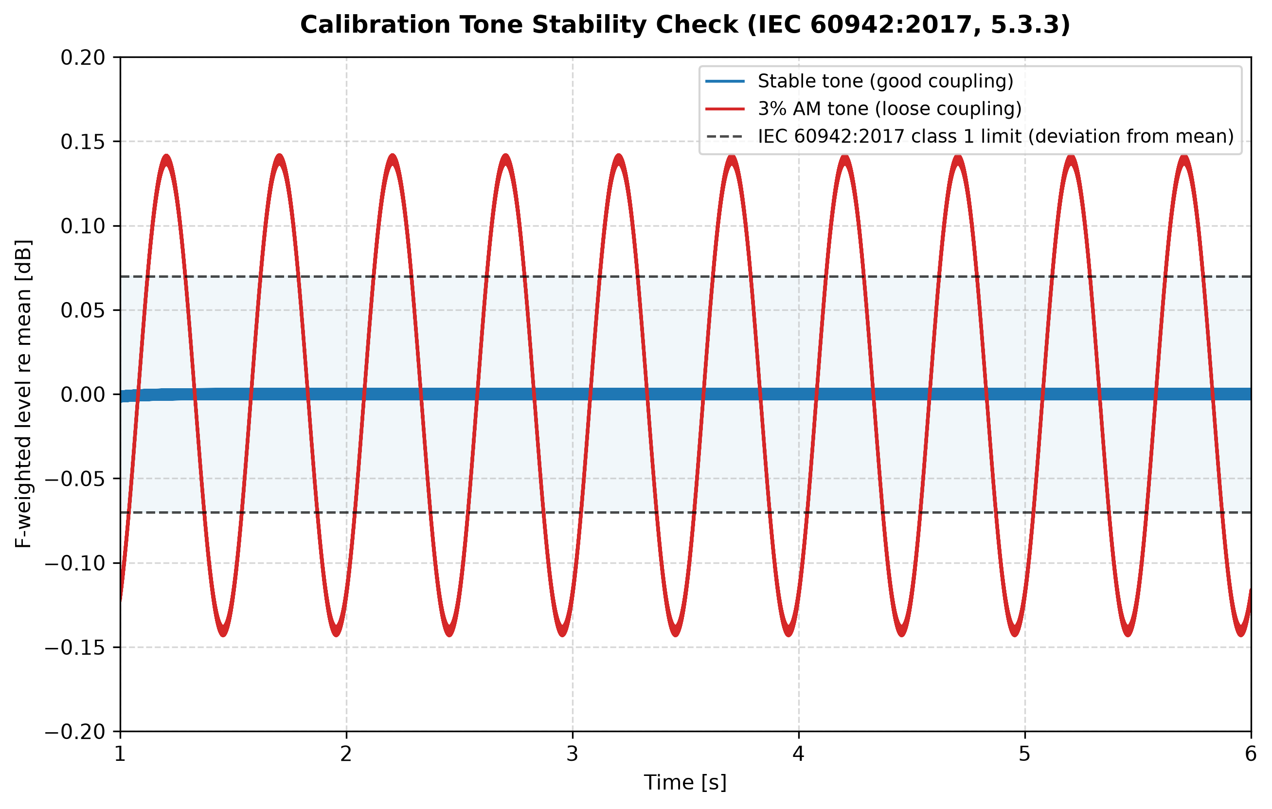
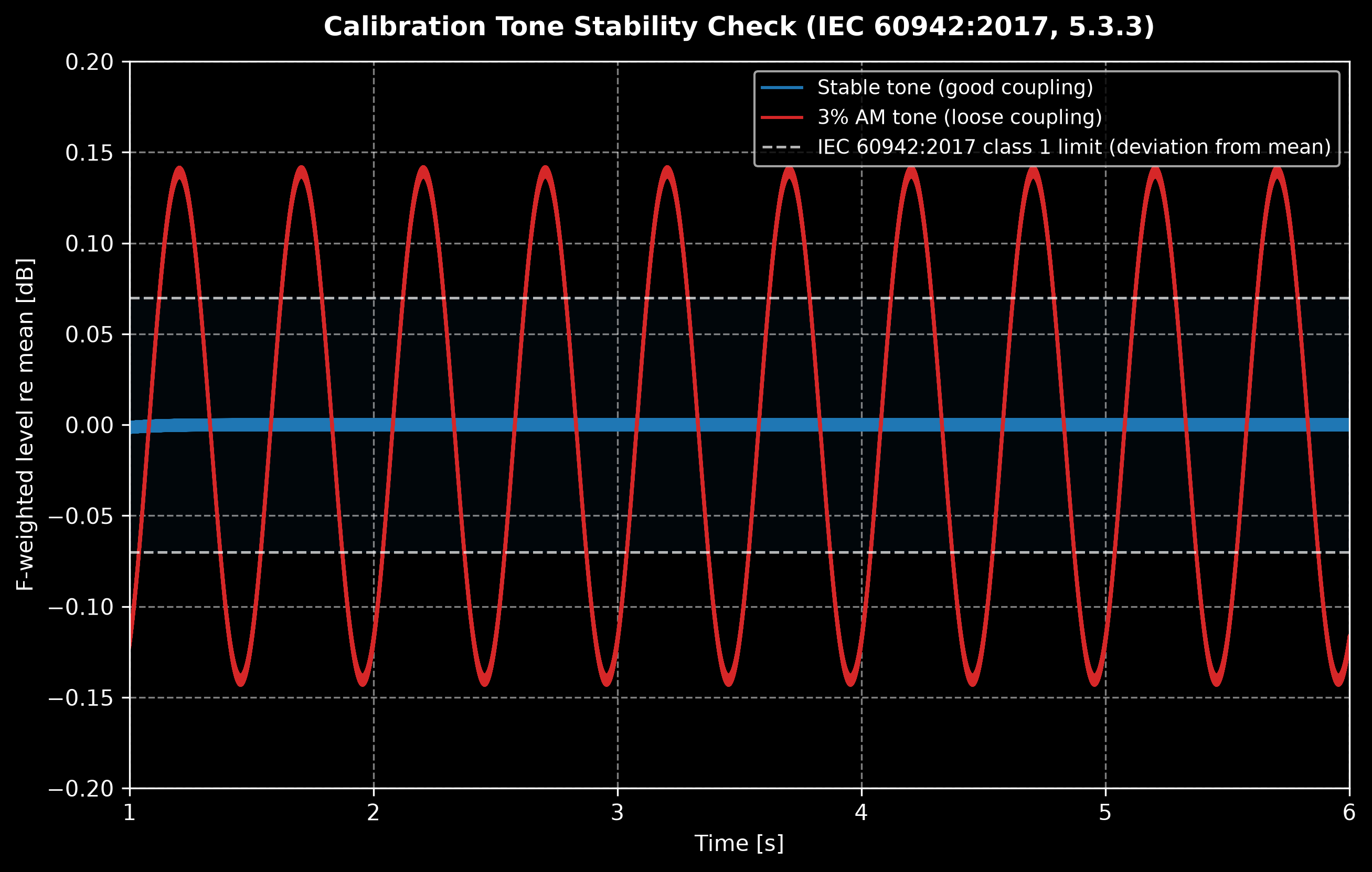
When you pass the sample rate (and validate=True, the default), sensitivity(ref, fs=fs) checks the recording the way IEC 60942:2017 checks the calibrator itself (5.3.3): the short-term level fluctuation, the absolute difference between each of the maximum and minimum F-time-weighted levels and the mean level, must not exceed the Table 2 class 1 limit for the calibrator’s nominal frequency (0.07 dB at and above 160 Hz, relaxed to 0.10 dB below 160 Hz and 0.20 dB at or below 63 Hz, where the F time-weighting itself ripples). Pass frequency= to select the right row for non-1 kHz calibrators. A CalibrationWarning flags badly coupled microphones or handling noise before they silently corrupt every calibrated level. The recording must be at least 2 s long (1 s for the F-integrator to settle plus 1 s of settled envelope); shorter recordings get a warning instead of an unreliable verdict. Without fs the check is skipped. Override the limit with max_fluctuation_db or disable with validate=False.

The check catches exactly what ruins field calibrations (a loose coupler, wind, handling noise):

Show the code for this figure

import matplotlib.pyplot as plt
import numpy as np
from phonometry import metrology

fs = 48000
t = np.arange(int(fs * 6.0)) / fs
stable = 0.5 * np.sin(2 * np.pi * 1000 * t)
# 3 % amplitude modulation at 2 Hz: ~0.14 dB of wobble, clearly over
unstable = stable * (1 + 0.03 * np.sin(2 * np.pi * 2.0 * t))

plt.figure(figsize=(9, 5))
skip = fs                     # discard the F-integrator attack (~8 tau)
for x, label in ((stable, "Stable tone (good coupling)"),
                 (unstable, "3% AM tone (loose coupling)")):
    env = metrology.time_weighting(x, fs, mode="fast")[skip:]
    level = 10 * np.log10(np.maximum(env, np.finfo(float).eps))
    plt.plot(t[skip:], level - level.mean(), label=label)
for lim in (0.07, -0.07):
    plt.axhline(lim, linestyle="--", color="gray")
plt.xlabel("Time [s]")
plt.ylabel("F-weighted level re mean [dB]")
plt.legend()
plt.show()

sensitivity() parameters

Parameter	Type / shape	Units	Range / default	Notes
ref_signal	1D/2D array	digital units	non-empty, non-silent	Recording of the calibration tone only (trim handling noise)
target_spl	float	dB re 20 µPa	default 94.0	The calibrator’s nominal level (114 dB calibrators: pass 114.0)
ref_pressure	float	Pa	default 2e-5	Reference pressure p₀; rarely changed
fs	int, optional	Hz	> 0; default None	Required for the stability validation; omit to skip it
validate	bool	—	default True	Emit CalibrationWarning on unstable/short recordings
max_fluctuation_db	float, optional	dB	default None → Table 2 class 1	Explicit override of the stability limit
frequency	float	Hz	default 1000.0	Calibrator’s nominal frequency; selects the IEC 60942 Table 2 row
narrowband	bool	—	default False	Estimate the tone with a coherent Goertzel detector near frequency (needs fs) instead of full-band RMS; rejects broadband hum/noise that otherwise inflates the RMS and shrinks every later level (~−0.44 dB at 20 dB SNR). Enable for noisy coupler recordings

Returns the sensitivity factor (float) to pass as calibration_factor= to octave_filter, leq, laeq, ln_levels, lc_peak, sel and the dose functions.

Field checks, laboratory verification and drift

Calibration lives at three time scales:

• Every session: the field check. Couple the calibrator and derive the sensitivity before each measurement series, and check it again at the end. Normative methods make the second check mandatory and use the pre/post difference as a validity gate (a common criterion invalidates the series when the two differ by more than 0.5 dB). Whatever the threshold, the difference is your drift bound for everything captured in between; carry it into the uncertainty budget rather than assuming zero.
• Periodically: laboratory verification. A field check only compares the chain against the calibrator; it cannot see an error the calibrator and meter share, and it says nothing about the response away from 1 kHz. IEC 61672-3 defines the periodic tests for the meter (weightings, level linearity and ballistics spot-checked against the class limits), and IEC 60942 the corresponding tests for the calibrator itself; typical laboratory intervals are one to two years.
• Between checks: drift. Microphone sensitivity moves with temperature, humidity and capsule aging; electronics with battery voltage. A healthy class 1 chain drifts a few hundredths of a dB over a session, which is why a pre/post difference of half a decibel signals damage rather than weather. The largest “drift” of all is a touched gain knob: the factor S is valid only while the chain stays exactly as calibrated.

One more class subtlety: tolerances chain. A class 1 measurement requires a class 1 (or LS) calibrator and a class 1 meter; calibrating a class 1 chain with a class 2 calibrator silently downgrades every derived level to class 2 accuracy, because the calibrator’s wider level tolerance enters S directly.

Digital Analysis (dBFS)

If you are working with digital audio files (e.g., WAV, FLAC) and want to analyze levels relative to Full Scale rather than physical pressure, you can use the dbfs=True parameter.

In this mode:

• 0 dBFS corresponds to a numeric signal level of 1.0 (RMS or Peak).
• calibration_factor does not apply (dBFS is relative to digital full scale).
• Useful for analyzing headroom, digital mastering, or normalized signals.

import numpy as np
from phonometry import metrology

fs = 48000
# recording: the mic capture you want to calibrate, same input chain (Pa after calibration).
#   Synthesized here; in a real measurement this is your recorded signal.
recording = 0.2 * np.sin(2 * np.pi * 1000 * np.arange(fs) / fs)

# Assume 'recording' is normalized between -1.0 and 1.0
spl_dbfs, freq = metrology.octave_filter(recording, fs, dbfs=True)
# Results will be negative (e.g., -20 dBFS)

RMS vs Peak Levels

phonometry supports two measurement modes to align with professional software like BK:

• RMS (mode='rms'): Energy-based level (standard).
• Peak (mode='peak'): Absolute maximum value reached in the frame (Peak-holding).

import numpy as np
from phonometry import metrology

fs = 48000
# recording: the mic capture you want to calibrate, same input chain (Pa after calibration).
#   Synthesized here; in a real measurement this is your recorded signal.
recording = 0.2 * np.sin(2 * np.pi * 1000 * np.arange(fs) / fs)

# Measure peak-holding levels for impact analysis
spl_peak, freq = metrology.octave_filter(recording, fs, mode='peak')

Note

mode='peak' measures the absolute maximum of the filtered band signal, which includes the filter’s onset transient (overshoot). Signals that start abruptly may read up to ~1 dB high. This is inherent to IIR band filters (an analog SLM behaves the same way), not a processing artifact.

Integer audio input

Integer signals (e.g. int16 from scipy.io.wavfile.read) are converted to float64 internally before any squaring, so calibration and level results are identical whether you pass the raw integer array or a float conversion.

What this guide covers

Covered. IEC 60942:2017 as far as it constrains the sensitivity factor: the principal calibrator level that target_spl assumes, the Table 1 class tolerances quoted in the uncertainty discussion above, and the short-term level-fluctuation check of clause 5.3.3 against the class 1 limits of Table 2, which sensitivity(ref, fs=fs) runs on the reference recording.

Not covered. The conformance tests of the calibrator itself (generated level, frequency, distortion, and the environmental corrections for static pressure and temperature) are not implemented, so pass an already corrected target_spl when the calibrator’s manual asks for one. The IEC 61672-3 periodic tests are cited as laboratory practice, not run: nothing here verifies a sound level meter or assigns it a class. The dBFS half of the page sits outside any standard and makes no physical claim.

See also

• Build a sound level meter: the walkthrough that starts from this calibration step and ends at a class-checked instrument.
• Levels: every metric that consumes the calibration_factor derived here.
• Multichannel and Performance: one sensitivity per channel when the channels differ.
• GUM uncertainty: propagating the calibrator tolerance and drift bound into a level’s uncertainty.
• API reference: metrology.calibration and phonometry.

Quick answers

What calibrator level should I use to calibrate my measurement chain?

The usual choice is 94 dB SPL at 1 kHz (1 Pa RMS), which is what sensitivity() assumes with its default target_spl=94.0; for a 114 dB calibrator pass 114.0. IEC 60942 requires the principal level to be at least 90 dB re 20 µPa. Record a few seconds of stable tone, because the standard specifies the generated level as a 20 s average.

How much drift between the pre and post calibration checks is acceptable?

Derive the sensitivity before each measurement series and check it again at the end: a common criterion invalidates the series when the two differ by more than 0.5 dB. A healthy class 1 chain drifts a few hundredths of a dB over a session, so a half-decibel pre/post difference signals damage rather than weather. Whatever the threshold, carry the difference into the uncertainty budget rather than assuming zero.

Can I calibrate a class 1 chain with a class 2 calibrator?

You can, but the tolerances chain: a class 1 measurement requires a class 1 (or LS) calibrator per IEC 60942 and a class 1 meter, so a class 2 calibrator silently downgrades every derived level to class 2 accuracy, because its wider level tolerance enters the sensitivity factor $S$ directly. For reference, the class 1 tolerance is ±0.4 dB between 160 Hz and 1.25 kHz (IEC 60942 Table 1).

References

• Bies, D. A., Hansen, C. H., & Howard, C. Q. (2017). Engineering noise control (5th ed.). CRC Press. https://doi.org/10.1201/9781351228152Sections 3.1.5 and 3.4 (microphone field effects and sound level meter calibration: the electrical and acoustic calibration practice this page's workflow follows). ISBN 978-1-4987-2405-0.
• International Electrotechnical Commission. (2013). Electroacoustics — Sound level meters — Part 3: Periodic tests (IEC 61672-3:2013). The laboratory verification procedure behind the recommended periodic checks.
• International Electrotechnical Commission. (2017). Electroacoustics — Sound calibrators (IEC 60942:2017). The calibrator level and class assumptions behind sensitivity() (the 94 dB principal level and the Table 1 class tolerances) and the short-term level-fluctuation stability check of the reference recording (clause 5.3.3, Table 2 class 1 limits per nominal frequency).