Time synchronous averaging

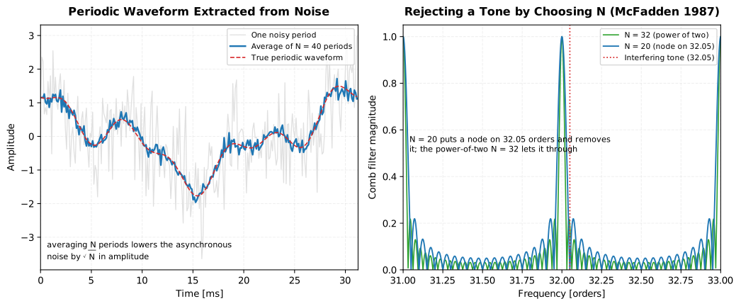
A rotating machine repeats its signature once per revolution. Buried in broadband noise and in the tones of every other shaft, that repetitive waveform is hard to read directly. Time synchronous averaging (TSA) recovers it: given the period T of one revolution, it slices the record into successive length-T blocks and averages them. Every component synchronous with T reinforces; everything asynchronous, noise and the harmonics of unrelated shafts, averages down. time_synchronous_average implements the model of P. D. McFadden, A revised model for the extraction of periodic waveforms by time domain averaging (1987).

Show the code for this figure

import matplotlib.pyplot as plt
import numpy as np
from phonometry import (
    comb_filter_response,
    noise_signal,
    time_synchronous_average,
)

fs = 8192.0
period = 1.0 / 32.0        # one revolution: 256 samples at this rate
m, n_avg = 256, 40
phase = np.arange((n_avg + 1) * m) / m
periodic = (
    np.cos(2.0 * np.pi * phase)
    + 0.5 * np.cos(2.0 * np.pi * 3.0 * phase + 0.4)
    - 0.3 * np.cos(2.0 * np.pi * 6.0 * phase)
)
recording = periodic + noise_signal(fs, phase.size / fs, rms=0.9, seed=11)
res = time_synchronous_average(recording, fs, period, n_averages=n_avg)

fig, (ax0, ax1) = plt.subplots(1, 2, figsize=(11, 4.6))
t_ms = 1e3 * res.times
ax0.plot(t_ms, recording[:m], color="#cccccc", label="One noisy period")
ax0.plot(t_ms, res.period_waveform, color="#1f77b4", lw=1.8,
         label=f"Average of N = {n_avg} periods")
ax0.plot(t_ms, periodic[:m], "--", color="#d62728", label="True waveform")
ax0.set_xlabel("Time [ms]"); ax0.set_ylabel("Amplitude"); ax0.legend()

orders = np.linspace(31.0, 33.0, 4000)
freqs = orders / period
ax1.plot(orders, comb_filter_response(freqs, period, 32), color="#2ca02c",
         label="N = 32 (power of two)")
ax1.plot(orders, comb_filter_response(freqs, period, 20), color="#1f77b4",
         label="N = 20 (node on 32.05)")
ax1.axvline(32.05, color="#d62728", ls=":", label="Interfering tone")
ax1.set_xlabel("Frequency [orders]"); ax1.set_ylabel("Comb filter magnitude")
ax1.set_ylim(0, 1.05); ax1.legend()
plt.show()

The .plot() method draws the averaged waveform and the comb filter in one call:

res.plot()          # English labels; res.plot(language="es") for Spanish

1. The average is a comb filter

Averaging N successive periods (McFadden Eq. 5),

$$a(t)=\frac{1}{N}\sum _{n=0}^{N-1}y(t+nT),$$

is, in the frequency domain, the multiplication of the signal spectrum by a comb filter (Eq. 8). Its magnitude (Eq. 9) is the Dirichlet kernel

$$|C(f)|=\left|\frac{\sin (N\pi fT)}{N\sin (\pi fT)}\right|.$$

The comb has a tooth of unit height at every harmonic k/T (the orders f·T = 1, 2, 3, ...), independent of N: components synchronous with the period pass untouched. Between the teeth it has nodes at j/(N·T) for every j that is not a multiple of N, where the response is exactly zero. comb_filter_response evaluates this closed form directly:

import numpy as np
from phonometry import comb_filter_response

period = 1.0 / 32.0
comb_filter_response(np.array([16.0 / period]), period, 8)   # 1.0 at a tooth
comb_filter_response(np.array([0.25 / period]), period, 2)   # 1/sqrt(2)
comb_filter_response(np.array([0.5 / period]), period, 2)    # 0.0 at a node

SynchronousAverageResult carries the response over the first few harmonics in comb_frequencies and comb_response, so the shape of the filter that the average applied is available alongside the recovered waveform.

2. Noise falls as the square root of the number of averages

Asynchronous noise of variance ${\sigma }^2$ averaged over N periods has residual variance ${\sigma }^2/N$: the residual standard deviation falls as $1/\sqrt{N}$, and the amplitude signal-to-noise ratio improves by $\sqrt{N}$. That is a power reduction of $10{\log }_{10}N$ dB, reported as noise_reduction_db, with the amplitude gain $\sqrt{N}$ as amplitude_snr_gain:

res = time_synchronous_average(recording, fs, period, n_averages=100)
res.noise_reduction_db      # 20.0 dB = 10*log10(100)
res.amplitude_snr_gain      # 10.0   = sqrt(100)
res.plot()                  # averaged waveform + the comb it applied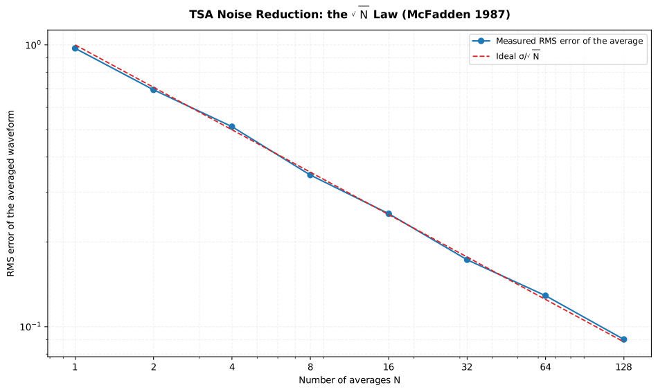

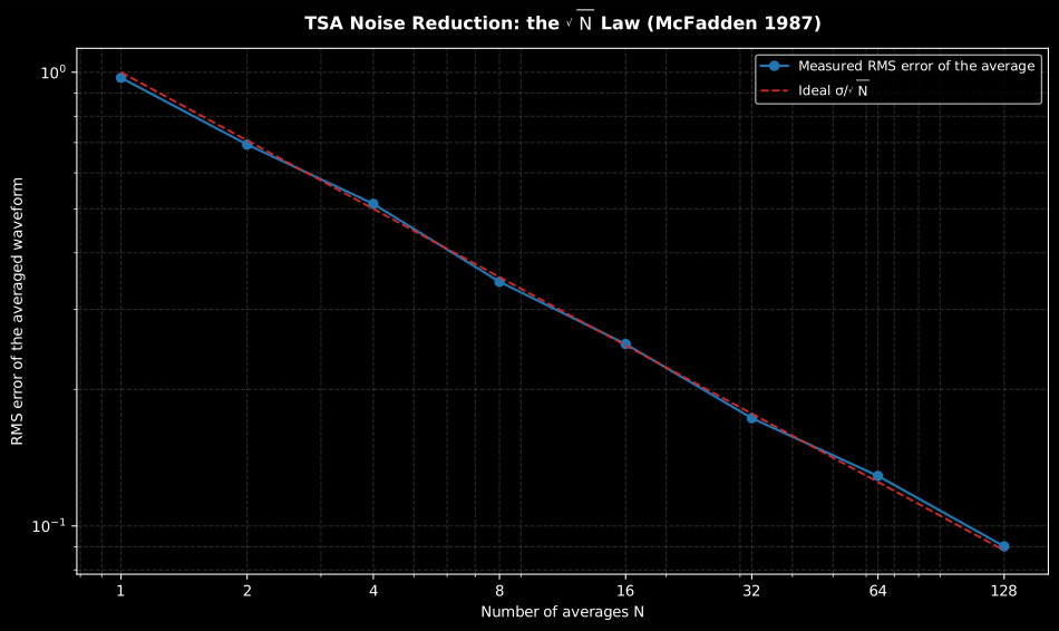
The √N law measured end to end: the RMS error of the averaged waveform of a three-harmonic gear signature in unit-variance noise falls along the ideal σ/√N line as the number of averaged periods grows from 1 to 128.

Show the code for this figure

import matplotlib.pyplot as plt
import numpy as np
from phonometry import time_synchronous_average

fs = 8192.0
samples = 256
period = samples / fs
m = np.arange(samples) / fs
true = (np.cos(2 * np.pi * m / period)
        + 0.5 * np.cos(2 * np.pi * 3 * m / period + 0.7)
        + 0.25 * np.cos(2 * np.pi * 5 * m / period + 1.1))
rng = np.random.default_rng(5)
recording = np.tile(true, 128) + rng.standard_normal(128 * samples)

counts = [1, 2, 4, 8, 16, 32, 64, 128]
errors = []
for n in counts:
    res = time_synchronous_average(recording[:n * samples], fs, period,
                                   n_averages=n)
    errors.append(np.sqrt(np.mean((res.period_waveform - true) ** 2)))

# One line — the averaged waveform and the comb filter it applied:
res.plot()
plt.show()

# The sqrt(N) law by hand: measured error against the ideal line:
fig, ax = plt.subplots()
ax.loglog(counts, errors, "o-", label="measured RMS error")
ax.loglog(counts, 1 / np.sqrt(np.array(counts)), "r--",
          label="ideal sigma/sqrt(N)")
ax.set(xlabel="Number of averages N", ylabel="RMS error")
ax.legend()
plt.show()

This law is the ideal one: it holds when the noise is uncorrelated from one period to the next, so colored or synchronous noise that is correlated across periods need not follow it. The residual (input minus the periodic reconstruction over the analysed span) and its residual_rms therefore report the noise actually left once the synchronous component is removed.

3. Choosing N to reject an interfering order

Because a tooth sits on every integer order, TSA passes the harmonics of the target shaft but also any tone that happens to fall on an integer order. A tone at a non-harmonic order q = f·T is only attenuated by the comb, not removed, and how much depends on where the nearest node lands. McFadden’s revised-model result is that such an interferer is best rejected by choosing N so that a node falls exactly on it, i.e. the smallest N with N·q an integer, rather than by the habitual power-of-two number of averages. An exact node exists only when the order q is rational, so some finite N makes N·q an integer; for an irrational or merely estimated order, choose the N whose node falls nearest the interfering order.

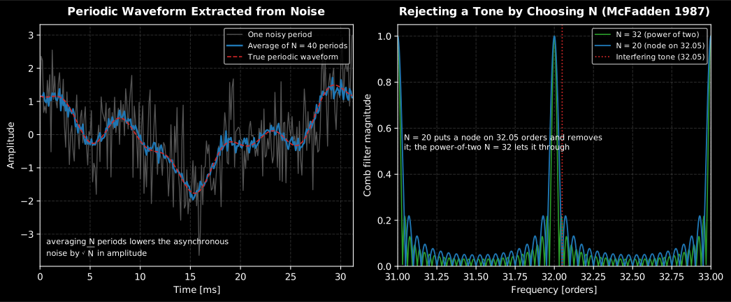
His own example is a tone at 32.05 orders. With N = 20 the product 20 · 32.05 = 641 is an integer, so a comb node lands on the tone and rejects it by more than 100 dB. The common choice N = 32 gives 32 · 32.05 = 1025.6, which sits on a side lobe: the tone is barely touched. The figure above shows both combs around order 32; the end-to-end average confirms it:

# true 8th-order component plus a strong interferer at 32.05 orders
phase = np.arange(41 * 256) / 256
recording = np.cos(2 * np.pi * 8.0 * phase) + 0.7 * np.cos(2 * np.pi * 32.05 * phase)

leak_20 = time_synchronous_average(recording, fs, period, n_averages=20)
leak_32 = time_synchronous_average(recording, fs, period, n_averages=32)
# leak_20.period_waveform matches the clean 8th-order tone; leak_32 does not

So a power-of-two number of averages, convenient as it is, is not in general the optimal choice: the interfering orders present in the machine should set N.

4. Non-integer samples per period

When fs·T is an integer, the period boundaries fall on samples, the blocks are sliced directly, and a noiseless periodic signal is recovered to machine precision (interpolated is False). When fs·T is not an integer the boundaries fall between samples; each block is then aligned to a common integer grid by the band-limited fractional delay of fractional_delay, and the waveform is recovered within that interpolation error (interpolated is True):

fs = 8192.0
period = 1.0 / 31.7                       # fs * period is not an integer
t = np.arange(int(40 * period * fs)) / fs
recording = np.cos(2.0 * np.pi * t / period)  # one cycle per revolution
res = time_synchronous_average(recording, fs, period)
res.interpolated                          # True: fractional-delay alignment
res.samples_per_period                    # integer samples of one period

By default the average uses as many whole periods as the record holds; pass n_averages to fix the count (for the node-selection choice of §3), and n_harmonics to set how many harmonics of 1/T the returned comb response spans.

The band-limited alignment shares its kernel with the sub-sample impulse-response alignment of the test-signals page, and the recovered waveform, being exactly one period, can be tiled to reconstruct the synchronous part of the signal for subtraction or for order analysis.

Which diagnostics tool, and when

TSA, the cepstrum and the envelope spectrum answer different questions about a rotating machine, and they compose rather than compete:

• TSA needs the period (a tacho pulse or a trusted shaft speed) and returns the waveform itself, one revolution of it: the tool when you want to see what a specific shaft or gear does per turn, tooth by tooth.
• The cepstrum needs no reference and detects any periodic family in the spectrum (harmonics, sidebands): the tool when the period is unknown or several families overlap and must be separated.
• The envelope spectrum finds periodicities of the amplitude: the tool for bearing-style faults, whose repetition rate modulates a high-frequency resonance instead of appearing as a low-frequency tone.

The composition is standard practice: average synchronously first, then subtract; the residual field is the record with the synchronous part removed, which is exactly what the envelope spectrum should be run on once the strong gear components no longer mask the modulation.

What this guide covers

Covered. McFadden’s revised model for time domain averaging (Mechanical Systems and Signal Processing, 1987): the comb-filter description of the average (Eq. 8, magnitude Eq. 9) implemented by comb_filter_response, the square-root noise-reduction law reported as noise_reduction_db and amplitude_snr_gain, and the choice of N that places a comb node on an interfering order, following the paper’s own 32.05-order example. time_synchronous_average also implements the band-limited fractional-delay alignment used when fs·T is not an integer.

Not covered. TSA needs a known period; finding that period, or detecting periodic families without one, is the job of the cepstrum, not of this page. Locating amplitude-modulation periodicities, such as bearing faults, is the envelope spectrum, also outside this page. McFadden’s paper is not a certification standard, so there is no compliance clause to check the implementation against.

See also

• Cepstrum and echoes: reference-free detection of harmonic and sideband families, and the envelope spectrum.
• Correlation and delay: the Hilbert envelope behind envelope analysis.
• Test signals: the fractional-delay kernel the non-integer period alignment uses.
• API reference: metrology.synchronous_average.

References

• McFadden, P. D. (1987). A revised model for the extraction of periodic waveforms by time domain averaging. Mechanical Systems and Signal Processing 1(1), 83-95. https://doi.org/10.1016/0888-3270(87)90043-2The comb-filter model of synchronous averaging (Eq. 8, magnitude Eq. 9), the revised finite-record model that yields an exactly periodic result, and the observation that a non-harmonic interfering order is best rejected by choosing the number of averages so that a comb node lands on it, not by the habitual power of two.