System measurement: Golay, shaped sweeps, inversion

The room-acoustics guide recovers impulse responses with the two ISO 18233 work-horses - the exponential sweep and the MLS. This page adds the measurement-engineering layer around them, from the transfer-function literature rather than a standard: complementary Golay pairs (a third excitation whose deconvolution is exactly free of correlation noise), shaped sweeps whose magnitude spectrum follows any prescribed target while keeping a swept sine’s crest factor, and the regularized inversion of a measured response - the tool that turns a measured loudspeaker or microphone response into a safe equalizer, and the bridge between the two: the inverse of a measured response is the natural target spectrum for the next measurement’s sweep.

1. Complementary Golay pairs

A Golay pair are two binary sequences a, b of length L = 2**n, built by a two-line recursion - append b to a, and -b to a (Havelock Part I Ch. 6, Eq. (1)). Their defining property is algebraic, not approximate: the two periodic autocorrelations sum to

$$\sum _j{a}_j{a}_{j+k}+b_j{b}_{j+k}=\{\begin{array}{ll}2L& k=0\\ 0& k\ne 0,\end{array}$$

an exact delta (Eq. (2)). An MLS autocorrelation has a -1 residue at every nonzero lag; the Golay sidelobes cancel identically. The measurement runs each code in turn - play a periodically, record one steady-state period, then the same with b - and sums the two circular cross-correlations (Eq. (4)): for a noiseless linear time-invariant system the impulse response comes back to machine precision, a closed-form identity the tests and the conformance report pin at 1e-13.

import numpy as np
from scipy import signal
from phonometry import golay_impulse_response, golay_pair

fs = 48000
pair = golay_pair(14)                       # two 16384-sample codes

# Simulated measurement: play each code periodically and record one
# steady-state period of a room-like band-pass system.
b, a = signal.butter(2, [80.0, 12000.0], btype="bandpass", fs=fs)
length = pair[0].size
rec_a = signal.lfilter(b, a, np.tile(pair[0], 3))[2 * length:]
rec_b = signal.lfilter(b, a, np.tile(pair[1], 3))[2 * length:]

ir = golay_impulse_response(rec_a, rec_b, pair, fs=fs)
print(ir.method, ir.size)                   # golay 16384
ir.plot()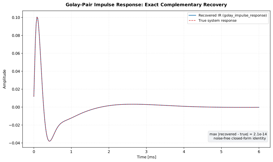

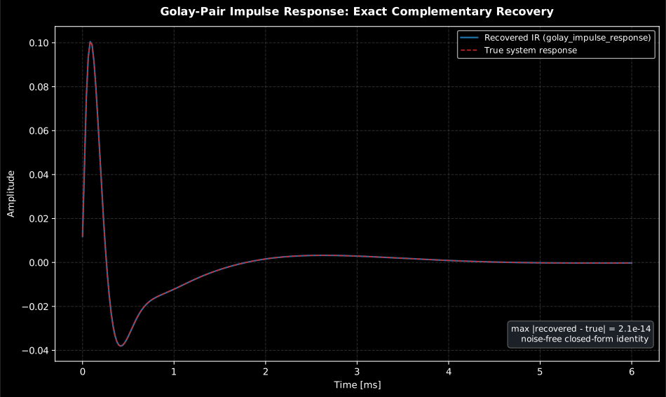
The Golay recovery of a band-pass system’s impulse response: the summed complementary correlations land on the true response to machine precision (max error 2·10⁻¹⁴ here), the closed-form identity the tests pin.

Show the code for this figure

import matplotlib.pyplot as plt
import numpy as np
from scipy import signal
from phonometry import golay_impulse_response, golay_pair

fs = 48000
pair = golay_pair(14)                       # two 16384-sample codes
b, a = signal.butter(2, [200.0, 2000.0], btype="bandpass", fs=fs)
length = pair[0].size
rec_a = signal.lfilter(b, a, np.tile(pair[0], 3))[2 * length:]
rec_b = signal.lfilter(b, a, np.tile(pair[1], 3))[2 * length:]

ir = golay_impulse_response(rec_a, rec_b, pair, fs=fs)

# One line — the recovered impulse response:
ir.plot()
plt.show()

# By hand, against the true system response:
impulse = np.zeros(length)
impulse[0] = 1.0
true_ir = signal.lfilter(b, a, impulse)
err = np.max(np.abs(np.asarray(ir) - true_ir))

t_ms = 1e3 * np.arange(length) / fs
view = t_ms <= 6.0
fig, ax = plt.subplots()
ax.plot(t_ms[view], np.asarray(ir)[view], label="Recovered IR")
ax.plot(t_ms[view], true_ir[view], "r--", label="True system response")
ax.set(xlabel="Time [ms]", ylabel="Amplitude",
       title=f"max |recovered - true| = {err:.1e}")
ax.legend()
plt.show()

The result is the same ImpulseResponseResult the sweep and MLS front ends return, so everything downstream - room parameters, decay curves, STI - consumes it unchanged. Recordings spanning several periods are synchronously averaged, so uncorrelated background noise falls by 3 dB per doubling while the deterministic part stays exact. The trade-offs mirror the MLS: the recovery is circular (the system must decay within one code period, or an ImpulseResponseWarning flags the aliased tail), distortion products smear across the period instead of separating like a sweep’s, and the two sequential steady states make the pair the most exposed of the family to time variance (Xiang’s Sec. 2) - the price of the exact complementarity.

2. Sweeps with an arbitrary target spectrum

A sweep’s energy at a given frequency can be set two ways: by its amplitude, or by how long it dwells there. Mueller & Massarani’s frequency-domain synthesis (Secs. 4.2-4.3) uses the second lever: define the target magnitude |H(f)|, make the group delay grow in proportion to the target’s power,

$${\tau }_G(f)={\tau }_G(f-df)+C|H(f){|}^2,C=\frac{{\tau }_G(f_{end})-{\tau }_G(f_{start})}{\sum |H(f){|}^2},$$

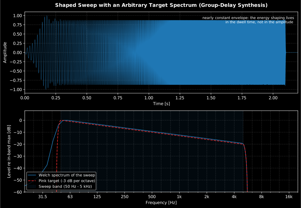
(Eqs. (11)-(12)), integrate the group delay into a phase, and inverse-FFT. The sweep then follows any spectral shape with a nearly constant envelope, keeping the crest factor close to a swept sine’s ideal 3.02 dB - unlike a noise signal with the same spectrum, which sits ~6 dB higher. shaped_sweep_signal implements the construction with the paper’s band-limiting and Nyquist-phase details; target is "pink" (the classical room-measurement emphasis, default), "white", or any (frequencies_hz, magnitude_db) pair:

from phonometry import shaped_sweep_signal

fs = 48000
sweep = shaped_sweep_signal(fs, 50.0, 5000.0, 2.0, target="pink")
print(round(sweep.crest_factor_db, 1))      # 4.2 (dB; the ideal is 3.02)
sweep.plot()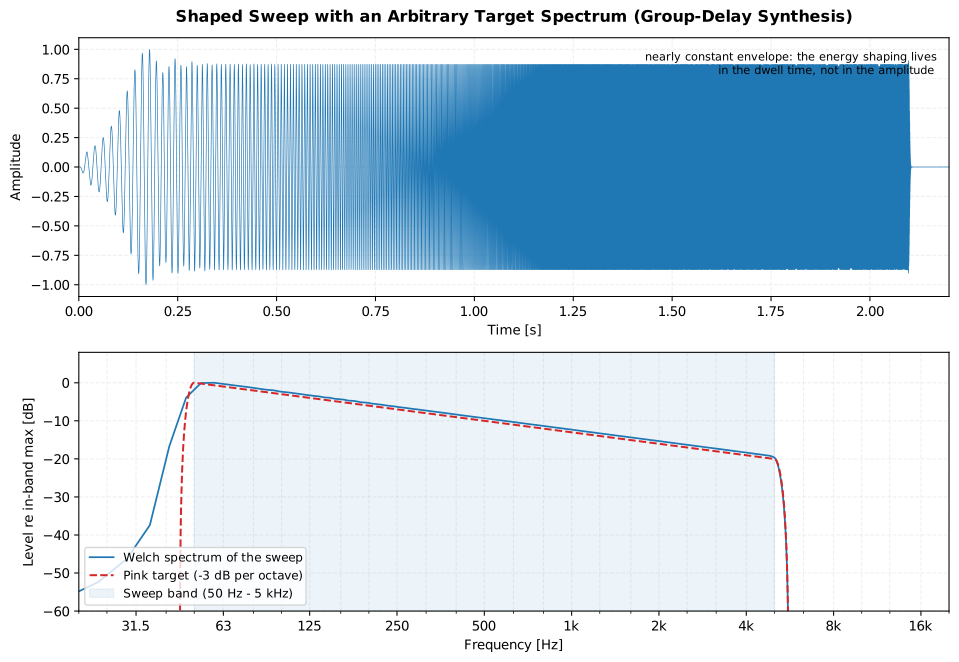

Show the code for this figure

import matplotlib.pyplot as plt
import numpy as np
from scipy import signal as sp_signal
from phonometry import shaped_sweep_signal

fs = 48000
res = shaped_sweep_signal(fs, 50.0, 5000.0, 2.0, target="pink")
x = np.asarray(res)

nperseg = 8192   # 75 % overlap: 50 % would ripple ~2 dB on a sweep
freqs, psd = sp_signal.welch(x, fs=fs, nperseg=nperseg,
                             noverlap=3 * nperseg // 4)
welch_db = 10.0 * np.log10(psd)
welch_db -= welch_db[(freqs >= 50.0) & (freqs <= 5000.0)].max()
target_db = 20.0 * np.log10(np.maximum(res.magnitude, 1e-300))
target_db -= target_db[(res.frequencies >= 50.0)
                       & (res.frequencies <= 5000.0)].max()

fig, axes = plt.subplots(2, 1, figsize=(10, 7))
axes[0].plot(np.arange(x.size) / fs, x, lw=0.5)
axes[0].set_xlabel("Time [s]")
axes[0].set_ylabel("Amplitude")
axes[1].semilogx(freqs[1:], welch_db[1:], lw=1.3, label="Welch spectrum")
axes[1].semilogx(res.frequencies[1:], target_db[1:], "r--",
                 label="Pink target (-3 dB per octave)")
axes[1].axvspan(50.0, 5000.0, alpha=0.08, label="Sweep band")
axes[1].set_xlabel("Frequency [Hz]")
axes[1].set_ylabel("Level re in-band max [dB]")
axes[1].set_ylim(-60.0, 8.0)
axes[1].legend()
plt.tight_layout()
plt.show()

The synthesis metadata travels with the result: frequencies and magnitude are the exact band-limited magnitude imposed on the spectrum, group_delay is the sweep’s time-frequency trajectory, and crest_factor_db the achieved peak-to-RMS ratio. The purpose of the shaping is signal-to-noise engineering: matching the emitted spectrum to the ambient noise floor (or to a loudspeaker’s power-handling limits) buys a frequency-independent SNR that no post-processing can recover (Mueller & Massarani Sec. 3).

Deconvolution needs nothing new - the result acts as its own reference array for the spectral method of impulse_response, which divides the sweep’s coloration out again:

import numpy as np
from scipy import signal
from phonometry import impulse_response, shaped_sweep_signal

fs = 48000
freqs = np.array([50.0, 200.0, 1000.0, 8000.0])
emphasis = np.array([12.0, 6.0, 0.0, 0.0])   # LF boost against rumble
sweep = shaped_sweep_signal(fs, 50.0, 8000.0, 3.0,
                            target=(freqs, emphasis))

# Simulated measurement of a known system (replace with play/record):
b, a = signal.butter(2, [200.0, 4000.0], btype="bandpass", fs=fs)
excitation = np.concatenate([np.asarray(sweep), np.zeros(fs)])
recorded = signal.lfilter(b, a, excitation)

ir = impulse_response(recorded, excitation, fs, length=fs)
ir.plot()

The emphasis re-weights the measurement’s noise floor, not the recovered response. One subtlety inherited from the hard band-limiting: the deconvolution’s band-limiting kernel is zero-phase, so a small anticausal tail sits at the very end of the full deconvolution buffer - keep return_full=True when hunting for tenth-of-a-dB accuracy at the band edges.

3. Regularized spectral inversion

Equalizing with a measured response means inverting it, and a plain reciprocal 1/H(f) explodes wherever the system radiates little energy - a notch in-band, everything out-of-band - turning an equalizer into a noise amplifier. Mueller & Massarani confine the inversion with a band-pass (Secs. 3.1, 4.5); the general form of that confinement is Kirkeby & Nelson’s frequency-dependent Tikhonov regularization,

$$H_{inv}(f)=\frac{H^{\ast }(f)}{|H(f){|}^2+\epsilon (f)},$$

with ε(f) small inside the band to be equalized and large outside. In-band the equalized magnitude |H·H_inv| deviates from unity by exactly ε/(|H|² + ε) - a closed form the conformance suite checks bin by bin - and out-of-band the filter gain can never exceed 1/(2·√ε), the analytic maximum of x/(x² + ε). A modeling delay of half the filter block makes the generally anticausal inverse of a mixed-phase response causal (Kirkeby & Nelson Sec. 2.4).

import numpy as np
from scipy import signal
from phonometry import regularized_inverse_filter

fs = 48000.0
# A loudspeaker-like measured response (replace with a measured IR).
b, a = signal.butter(2, [100.0, 8000.0], btype="bandpass", fs=fs)
imp = np.zeros(2048)
imp[0] = 1.0
h = signal.lfilter(b, a, imp)

inv = regularized_inverse_filter(h, fs, f_range=(200.0, 4000.0))
print(round(inv.flatness_db, 5))    # 1e-05 (dB: in-band deviation from 0 dB)
print(round(inv.max_gain_db, 1))    # -6.0 (dB: capped out-of-band boost)
inv.plot()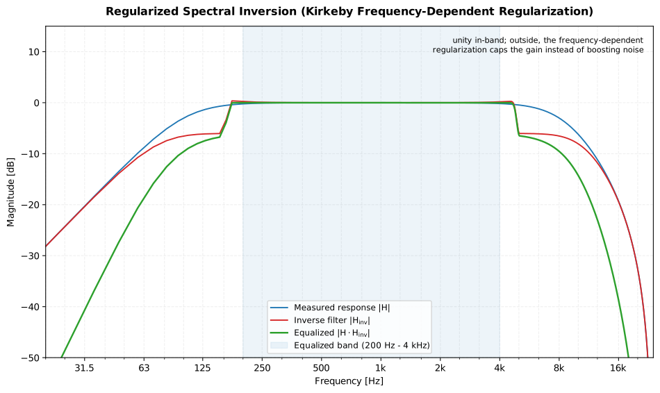

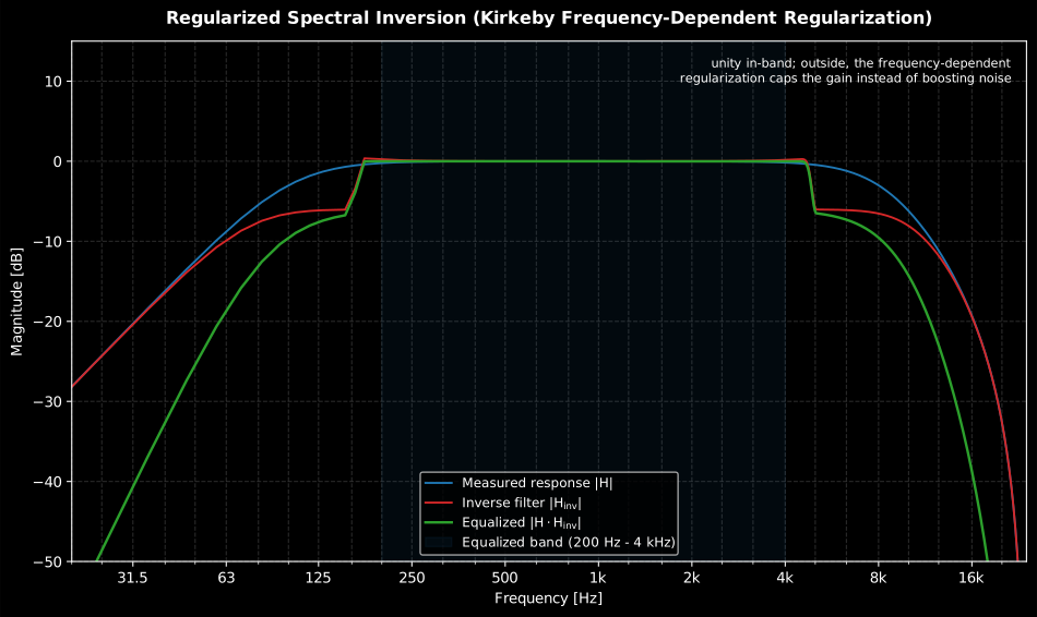
Show the code for this figure

import matplotlib.pyplot as plt
import numpy as np
from scipy import signal
from phonometry import regularized_inverse_filter

fs = 48000.0
b, a = signal.butter(2, [100.0, 8000.0], btype="bandpass", fs=fs)
imp = np.zeros(2048)
imp[0] = 1.0
h = signal.lfilter(b, a, imp)

res = regularized_inverse_filter(h, fs, f_range=(200.0, 4000.0))
f = res.frequencies[1:]
h_mag = np.abs(res.response_spectrum)[1:]
inv_mag = np.abs(res.spectrum)[1:]
peak = h_mag.max()

fig, ax = plt.subplots(figsize=(10, 6))
ax.semilogx(f, 20 * np.log10(h_mag / peak), label="Measured $|H|$")
ax.semilogx(f, 20 * np.log10(inv_mag * peak),
            label=r"Inverse $|H_{\mathrm{inv}}|$")
ax.semilogx(f, 20 * np.log10(h_mag * inv_mag), lw=1.8,
            label=r"Equalized $|H \cdot H_{\mathrm{inv}}|$")
ax.axvspan(200.0, 4000.0, alpha=0.08, label="Equalized band")
ax.set_ylim(-50.0, 15.0)
ax.set_xlabel("Frequency [Hz]")
ax.set_ylabel("Magnitude [dB]")
ax.legend()
plt.show()

Both regularization levels are fractions of the peak of |H|², generalising the scalar regularization of impulse_response: regularization_inside (default 1e-6) sets how exactly the band is flattened, regularization_outside (default 1.0) caps the out-of-band boost 6 dB below the in-band unity, and a geometric cross-fade over transition_octaves (default 1/3) connects the two smoothly. The result’s apply() equalizes any recording with the modeling delay already removed, and the function accepts an ImpulseResponseResult directly - its sample rate rides along:

import numpy as np
from scipy import signal
from phonometry import (impulse_response, regularized_inverse_filter,
                        sweep_signal)

fs = 48000
sweep = sweep_signal(fs, 50.0, 20000.0, 1.0)
excitation = np.concatenate([sweep, np.zeros(fs // 2)])
b, a = signal.butter(2, [100.0, 8000.0], btype="bandpass", fs=fs)
recorded = signal.lfilter(b, a, excitation)     # play/record in reality

ir = impulse_response(recorded, excitation, fs)  # any front end works
inv = regularized_inverse_filter(ir, f_range=(200.0, 10000.0))
flat_recording = inv.apply(recorded)             # delay already removed
inv.plot()   # measured, inverse and equalized magnitudes (figure above)

Closing the loop: pre-emphasis from a measured response

The two halves of this page compose into Mueller & Massarani’s own workflow (their Fig. 18): measure the loudspeaker, invert its response in the transmission band, and hand the inverse magnitude to the sweep synthesis as the target - the next measurement then radiates a flat acoustic spectrum, with the equalization done by the excitation instead of by noise-amplifying post-processing:

import numpy as np
from scipy import signal
from phonometry import regularized_inverse_filter, shaped_sweep_signal

fs = 48000.0
b, a = signal.butter(2, [100.0, 8000.0], btype="bandpass", fs=fs)
imp = np.zeros(2048)
imp[0] = 1.0
h = signal.lfilter(b, a, imp)                    # the measured response

inv = regularized_inverse_filter(h, fs, f_range=(200.0, 4000.0))
target_db = 20.0 * np.log10(
    np.abs(inv.spectrum[1:]) * np.abs(inv.response_spectrum).max()
)
sweep = shaped_sweep_signal(int(fs), 200.0, 4000.0, 3.0,
                            target=(inv.frequencies[1:], target_db))
sweep.plot()   # waveform and spectrum against the inverted-response target

Relation to the other tools

The Golay pair joins sweep_signal and mls_signal in the ISO 18233 acquisition family; pick the sweep for distortion rejection, the MLS for legacy hardware, the pair when exact noise-free deconvolution of a time-invariant system matters (HRTF rigs, calibration fixtures). Harmonic analysis of what sweeps discard lives in swept-sine distortion. The Welch machinery used to verify the shaped sweep is the calibrated spectral analysis page, and the equalized responses feed the same downstream chain as every impulse response.

What this guide covers

Covered. The complementary Golay pair (Golay 1961; Havelock, Kuwano & Vorländer eds., 2008, Part I Ch. 6 by Xiang): the append recursion, the exact complementary-autocorrelation identity and the summed-correlation recovery, implemented by golay_pair and golay_impulse_response. The group-delay sweep synthesis of Müller & Massarani (2001, Secs. 4.2-4.3), implemented by shaped_sweep_signal. The frequency-dependent Tikhonov regularization of Kirkeby & Nelson (1999, Eq. 17 and Sec. 2.4), implemented by regularized_inverse_filter.

Not covered. These are measurement-engineering methods from the transfer-function literature, not a certification standard, so there is no compliance clause to check against. Kirkeby & Nelson’s original inversion targets multi-loudspeaker sound reproduction, with a matrix regularization for crosstalk cancellation between several channels. regularized_inverse_filter implements only the single-channel, scalar case of their Eq. 17.

References

• Golay, M. J. E. (1961). Complementary series. IRE Transactions on Information Theory, 7(2), 82-87. https://doi.org/10.1109/TIT.1961.1057620The original construction of the complementary pairs of §1.
• Havelock, D., Kuwano, S., & Vorländer, M. (eds.). (2008). Handbook of signal processing in acoustics. Springer. https://doi.org/10.1007/978-0-387-30441-0Part I Chapter 6 (Xiang, Digital Sequences): the Golay recursion of §1, the complementary-autocorrelation identity of Eq. (2) and the frequency-domain recovery procedure of Eq. (4) and Fig. 2. ISBN 978-0-387-77698-9.
• Kirkeby, O., & Nelson, P. A. (1999). Digital filter design for inversion problems in sound reproduction. Journal of the Audio Engineering Society, 47(7/8), 583-595. The frequency-dependent Tikhonov regularization of §3 (their Eq. (17)) and the modeling delay that makes the mixed-phase inverse causal (Sec. 2.4).
• Müller, S., & Massarani, P. (2001). Transfer-function measurement with sweeps. Journal of the Audio Engineering Society, 49(6), 443-471. The sweep-synthesis chapter behind §2: frequency-domain construction from magnitude and group delay (Sec. 4.2), the group-delay recursion for arbitrary magnitude spectra (Sec. 4.3, Eqs. (11)-(12)) and the band-limited inversion discussion of Secs. 3.1 and 4.5. The extended "Director's Cut" edition was consulted.