Spherical ground effect and advanced barriers

The ISO 9613-2 general method folds the ground and barrier terms into tabulated, energy-based corrections. This page covers the underlying wave acoustics in phonometry.environmental.ground_barriers: the spherical-wave reflection coefficient of a finite-impedance ground (Weyl-Van der Pol) and the wave-theoretic diffraction of a screen, both in a homogeneous (non-refracting, non-turbulent) atmosphere. These are the physical core of the Nord2000 / CNOSSOS ground and barrier models, and they resolve the frequency-dependent interference structure the octave-band Agr/Dz terms smooth away.

1. Spherical-wave ground effect (Weyl-Van der Pol)

The sound field of a point source above a locally reacting ground is the sum of a direct wave and a reflected wave weighted by the spherical-wave reflection coefficient Q (Attenborough Eq. 2.40a; Salomons Eq. 3.2):

$$p=\frac{e^{ik{R}_1}}{4\pi R_1}+Q\frac{e^{ik{R}_2}}{4\pi R_2},$$

with R1 the source-receiver distance and R2 the image-source distance. The coefficient (Attenborough Eq. 2.40c; Salomons Eq. D.58) corrects the plane-wave coefficient Rp for the curvature of the wavefront:

$$Q=R_p+(1-R_p)F(w),R_p=\frac{Z\cos \theta -1}{Z\cos \theta +1},$$ $$F(w)=1+i\sqrt{\pi }w{e}^{-w^2}\mathrm{erfc}(-iw),w=\sqrt{\frac{ik{R}_2}{2}}\left(\cos \theta +\frac{1}{Z}\right).$$

Here Z is the ground surface impedance normalized by ρc, θ is the angle of incidence from the ground normal (cos θ = (hs + hr)/R2), and the boundary-loss factor F(w) is written through the scaled complementary error function e^{-w²} erfc(-iw), i.e. the Faddeeva function scipy.special.wofz. The second term of Q is the ground wave that keeps the field finite at grazing incidence, where Rp → -1 and a plane-wave model would predict silence (Salomons Eqs. D.57, D.59, D.60).

The relative sound level (the excess attenuation, dB re free field) is (Salomons Eq. 3.4):

$$\Delta L=20\lg \left|1+Q\frac{R_1}{R_2}{e}^{ik(R_2-R_1)}\right|.$$

import numpy as np
from phonometry import ground_effect

bands = np.array([63., 125., 250., 500., 1000., 2000., 4000., 8000.])

# Grassland (effective flow resistivity sigma = 200 kPa.s/m^2), source 1 m and
# receiver 1.5 m high, 50 m apart. The impedance comes from the Delany-Bazley
# porous model of phonometry.materials (a semi-infinite ground).
res = ground_effect(bands, 1.0, 1.5, 50.0, flow_resistivity=2e5)
print(res.excess_attenuation)     # the ground dip (dB re free field)
print(res.reflection_coefficient) # complex Q per band
res.plot()                        # excess attenuation vs frequency

The ground impedance is either derived from an effective flow_resistivity (via the delany_bazley or miki model of phonometry.materials, which model a semi-infinite porous ground) or supplied directly as a normalized complex impedance (a scalar, per-band array, or a PorousMediumResult). A plain impedance value is taken in the e^{-iωt} convention of Salomons, in which a passive ground has Im(Z) > 0; the porous models of phonometry.materials work in the opposite e^{+jωt} convention (Im(Z) < 0), so anything obtained from them (a flow_resistivity or a PorousMediumResult) is conjugated internally before it enters the Weyl-Van der Pol formulas.

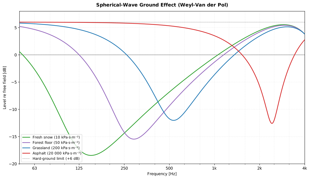
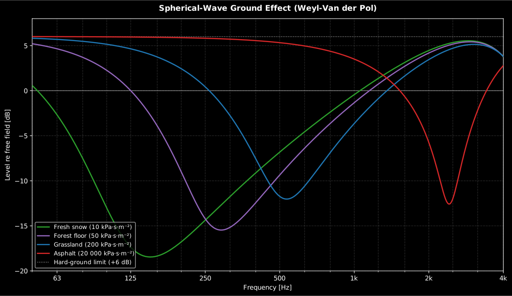
Show the code for this figure

import matplotlib.pyplot as plt
import numpy as np
from phonometry import ground_effect

freqs = np.geomspace(50.0, 4000.0, 400)
grounds = [
    ("Fresh snow (10 kPa)", 10e3, "#2ca02c"),
    ("Forest floor (50 kPa)", 50e3, "#9467bd"),
    ("Grassland (200 kPa)", 200e3, "#1f77b4"),
    ("Asphalt (20000 kPa)", 20000e3, "#d62728"),
]
fig, ax = plt.subplots(figsize=(11, 6.4))
for label, sigma, color in grounds:
    res = ground_effect(freqs, 1.0, 1.5, 50.0, flow_resistivity=sigma)
    ax.plot(freqs, res.excess_attenuation, color=color, label=label)
ax.axhline(6.0, color="k", ls=":", label="Hard-ground limit (+6 dB)")
ax.axhline(0.0, color="k", lw=0.8)
ax.set_xscale("log")
ax.set_xlabel("Frequency [Hz]")
ax.set_ylabel("Level re free field [dB]")
ax.legend()
plt.show()

Limits reproduced by the implementation (each a pinned test or conformance anchor): an acoustically hard ground (|Z| → ∞) gives Rp → 1, |w| → 0, F → 1 and Q → 1, so ΔL reaches +6 dB in phase; the effective flow resistivity σ → ∞ tends to that hard ground; grazing incidence (hs, hr → 0) gives Rp → -1; and the ground effect is reciprocal under an exchange of source and receiver heights.

2. Advanced barrier diffraction

Three levels of screening beyond the ISO 9613-2 Dz term are provided by barrier_insertion_loss and its building blocks.

Kurze-Anderson closed form. The insertion loss of a thin screen as a function of the Fresnel number N = (2/λ)(A + B − d) (Bies Eq. 5.134, with A and B the two segments of the shortest source-edge-receiver path and d the straight distance) is (Bies Eq. 5.138; Kurze & Anderson 1971):

$$\Delta =5+20\lg \left(\frac{\sqrt{2\pi N}}{\tanh \sqrt{2\pi N}}\right)\text{dB},$$

which tends to 5 dB at the shadow boundary N → 0 and approximates Maekawa’s point-source curve within about 1.5 dB.

from phonometry import barrier_insertion_loss, kurze_anderson_attenuation

kurze_anderson_attenuation(0.0)     # 5.0 dB at the shadow boundary

# A 4 m barrier 50 m from a 1 m source, receiver 1.5 m high at 100 m.
il = barrier_insertion_loss(bands, 1.0, 50.0, 4.0, 100.0, 1.5,
                            method="kurze_anderson")
il.plot()                           # insertion loss vs frequency

Exact rigid half-plane. With method="exact" the wave-theoretic insertion loss of a rigid thin screen is used: the compact Fresnel-integral form of the MacDonald / Hadden & Pierce solution (Attenborough Eqs. 9.19-9.20), built from the auxiliary Fresnel functions. It gives 6 dB at the shadow boundary (the field is exactly halved, the flat-wedge limit) and tracks Kurze-Anderson through the shadow zone.

Thick barriers. A thickness (top width e) lengthens the diffracted path to A + e + B, the double-edge Fresnel number N = (2/λ)(A + B + e − d) of Bies Eq. 5.157, so a thick barrier or a soil mound attenuates monotonically more than the thin screen of the same height.

Coherent barrier on the ground. With a ground_impedance (or a ground_flow_resistivity) the four source-image / receiver-image diffracted paths are combined coherently, each ground reflection weighted by the spherical-wave coefficient Q above (Attenborough Ch. 9; Bies Sec. 5.3.5). This exposes the ground-barrier interference structure that a purely energetic sum of Agr and Dz cannot. As a first-order simplification a single Q (over the overall source-receiver geometry) weights every bounce rather than a separate coefficient per image path; the model is coherent and reciprocal but not a full boundary-element solution.

il = barrier_insertion_loss(bands, 1.0, 50.0, 4.0, 100.0, 1.5,
                            method="exact", ground_flow_resistivity=2e5)
il.ground        # True: the four-path coherent ground model was applied
il.plot()

The three models side by side on the same geometry tell the whole story: the Kurze-Anderson fit and the exact half-plane track each other to within about 1.5 dB across two decades of Fresnel number, while the coherent ground model swings tens of decibels around them, up where the barrier removes the ground-effect dip of the unscreened path, down where the four diffracted paths interfere destructively.

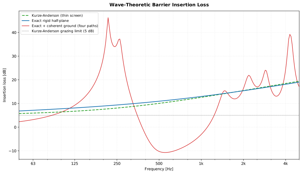
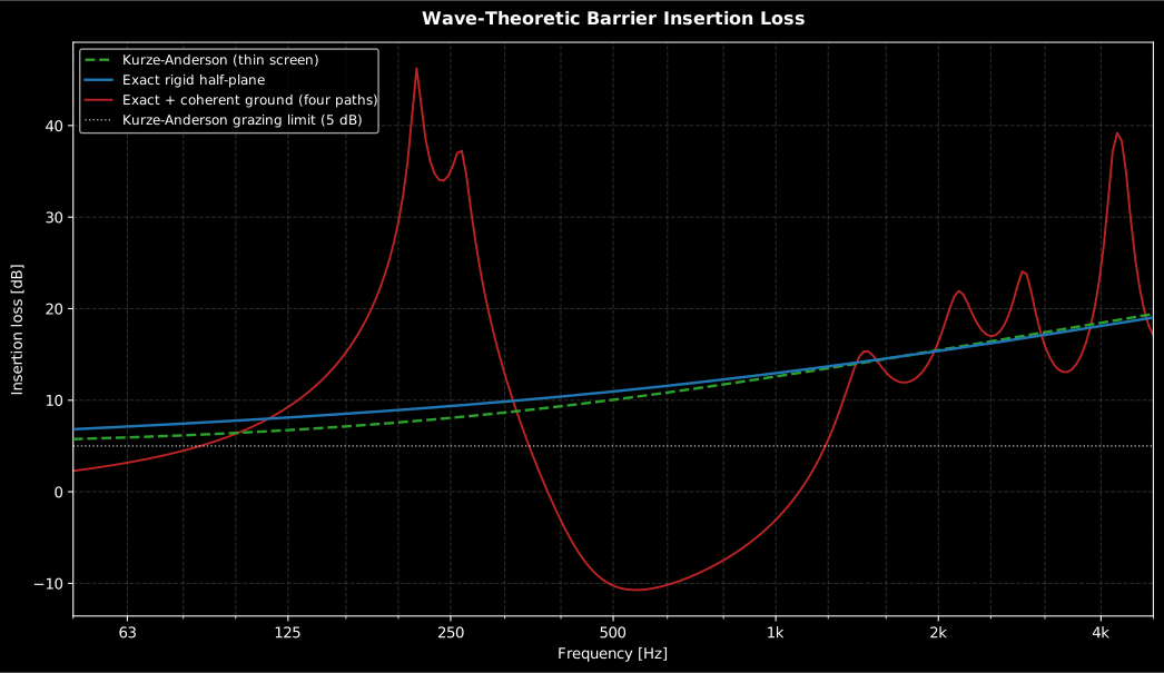
Show the code for this figure

import matplotlib.pyplot as plt
import numpy as np
from phonometry import barrier_insertion_loss

# The 4 m barrier of the snippets above, on a fine frequency grid.
freqs = np.geomspace(50.0, 5000.0, 240)
il_ka = barrier_insertion_loss(freqs, 1.0, 50.0, 4.0, 100.0, 1.5,
                               method="kurze_anderson")
il_ex = barrier_insertion_loss(freqs, 1.0, 50.0, 4.0, 100.0, 1.5,
                               method="exact")
il_gr = barrier_insertion_loss(freqs, 1.0, 50.0, 4.0, 100.0, 1.5,
                               method="exact", ground_flow_resistivity=2e5)
fig, ax = plt.subplots(figsize=(11, 6.4))
ax.semilogx(freqs, il_ka.insertion_loss, "--", label="Kurze-Anderson (thin screen)")
ax.semilogx(freqs, il_ex.insertion_loss, label="Exact rigid half-plane")
ax.semilogx(freqs, il_gr.insertion_loss, label="Exact + coherent ground (four paths)")
ax.axhline(5.0, color="k", ls=":", label="Kurze-Anderson grazing limit (5 dB)")
ax.set(xlabel="Frequency [Hz]", ylabel="Insertion loss [dB]")
ax.legend()
plt.show()

Relation to ISO 9613-2

The tabulated Agr and Dz of the ISO 9613-2 method are octave-band, energy-based engineering fits; ground_effect and barrier_insertion_loss are their narrowband wave-acoustic counterparts. Over hard ground both agree on the +6 dB enhancement and the 5 dB grazing barrier floor, but only the wave models resolve the interference dips that move with geometry, frequency and ground impedance, which is why they are the natural infrastructure for the meteorological schemes of Nord2000 and CNOSSOS.

What this guide covers

Covered. The Weyl-Van der Pol spherical-wave ground reflection coefficient (ground_effect, Attenborough Eq. 2.40a/c, Salomons Eq. 3.2/D.58, the Faddeeva-function boundary-loss factor), with its hard-ground +6 dB, grazing-incidence and reciprocity limits pinned as tests. Wave-theoretic barrier diffraction (barrier_insertion_loss): the Kurze-Anderson closed form (kurze_anderson_attenuation, Bies Eq. 5.138), the exact rigid half-plane (MacDonald / Hadden & Pierce, Attenborough Eqs. 9.19-9.20), thick barriers through the double-edge Fresnel number (Bies Eq. 5.157), and the coherent four-path barrier-on-ground model weighted by the ground_effect reflection coefficient.

Not covered. Both models assume a homogeneous, non-refracting, non-turbulent atmosphere; a vertical sound-speed gradient is the subject of the separate atmospheric refraction guide instead. The coherent barrier-on-ground model weights all four diffracted paths with a single reflection coefficient Q computed over the overall source-receiver geometry rather than a separate coefficient per image path, so it is coherent and reciprocal but not a full boundary-element solution.

References

• Attenborough, K., & Van Renterghem, T. (2021). Predicting outdoor sound (2nd ed.). CRC Press. https://doi.org/10.1201/9780429470141Chapter 2 (spherical-wave reflection over an impedance ground, the Weyl-Van der Pol equation and the boundary-loss factor) and Chapter 9 (outdoor noise barriers, the MacDonald and Hadden & Pierce diffraction solutions). ISBN 978-1-138-30655-2.
• Bies, D. A., Hansen, C. H., & Howard, C. Q. (2017). Engineering noise control (5th ed.). CRC Press. Sections 5.2.3 (spherical-wave ground reflection) and 5.3.5-5.3.7 (Fresnel number, Kurze-Anderson, thin- and thick-barrier diffraction). ISBN 978-1-4987-2405-0.
• Hadden, W. J., & Pierce, A. D. (1981). Sound diffraction around screens and wedges for arbitrary point source locations. Journal of the Acoustical Society of America, 69(5), 1266-1276. https://doi.org/10.1121/1.385809The exact wedge-diffraction solution whose flat-wedge (thin-screen) limit the barrier insertion loss uses.
• Kurze, U. J., & Anderson, G. S. (1971). Sound attenuation by barriers. Applied Acoustics, 4(1), 35-53. https://doi.org/10.1016/0003-682X(71)90024-7The closed-form fit to Maekawa's chart in the Fresnel number.
• Salomons, E. M. (2001). Computational atmospheric acoustics. Kluwer Academic. https://doi.org/10.1007/978-94-010-0660-6Chapter 3 and Appendix D: the two-ray field, the plane- and spherical-wave reflection coefficients, and the numerical distance (Eqs. D.57-D.60). ISBN 978-1-4020-0390-5.