Aircraft noise: Effective Perceived Noise Level

The Effective Perceived Noise Level (EPNL) is the noise-certification metric for transport-category aircraft. It condenses a half-second one-third-octave spectral time history of a flyover into a single number, in EPNdB, through five steps of ICAO Annex 16, Vol. I, Appendix 2. This page covers the four primitives that build the metric and the IEC 61265 measurement-system verifier. Each quantity is validated against the worked examples of the ICAO Doc 9501 Environmental Technical Manual (ETM) Vol. I.

Perceived noisiness and PNL

Each of the 24 one-third-octave-band levels (50 Hz–10 kHz) is converted to a perceived noisiness in noys by the analytic piecewise law of Table A2-3, then combined into the total noisiness N = 0.85·n_max + 0.15·Σn and the perceived noise level PNL = 40 + (10/lg2)·lg N.

from phonometry import aircraft

noys = aircraft.perceived_noisiness(spl)      # per-band noys (spl = 24 band levels, dB)
pnl = aircraft.perceived_noise_level(spl)      # PNdB

Tone correction

Spectral irregularities (fan/turbine tones) are penalised by a tone correction C, found with the slope (“encircling”) method: slopes are smoothed to a background spectrum SPL'', the tone excess F = SPL − SPL'' above 1.5 dB is mapped to a correction factor (frequency-split at 500 Hz / 5000 Hz, capped at 6⅔ dB), and the maximum over bands is taken. The implementation reproduces the ICAO Doc 9501 ETM Vol. I Table 3-7 turbofan example exactly (C = 2.0 dB at 2500 Hz).

from phonometry import aircraft

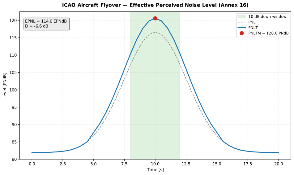
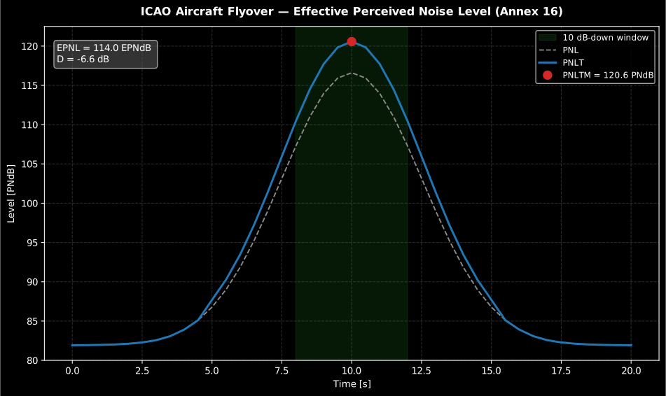
c = aircraft.tone_correction(spl)              # dB; added to PNL to give PNLT

EPNL

Over the flyover, PNLT = PNL + C, its maximum is PNLTM, and the metric integrates PNLT over the 10 dB-down window (the records nearest to PNLTM − 10 on each side) normalised to 10 s, so EPNL = PNLTM + D with the duration correction D.

from phonometry import aircraft

# spectra: a (K, 24) array of one-third-octave band levels sampled every dt s
res = aircraft.effective_perceived_noise_level(spectra, dt=0.5)
print(res.epnl, res.pnltm, res.duration_correction, res.band_limits)
res.plot()   # PNL/PNLT time history (needs matplotlib)

effective_perceived_noise_level returns an EPNLResult bundling the per-record pnl, tone_correction, pnlt, the peak pnltm, the duration_correction, the epnl and the 10 dB-down band_limits. The reference-condition integrated-method example of ETM Vol. I Table 4-4 is reproduced as EPNL = 92.6 EPNdB.

Show the code for this figure

import numpy as np
from phonometry import aircraft

k, dt = 41, 0.5
idx = np.arange(k)
shape = 15.0 * np.exp(-((np.log10(aircraft.NOY_BANDS) - np.log10(400.0)) ** 2) / 0.5)
gain = 30.0 * np.exp(-((idx - 20.0) ** 2) / (2 * 5.0**2)) - 5.0
spectra = (55.0 + shape)[None, :] + gain[:, None]
spectra[:, 17] += 12.0 * np.exp(-((idx - 20.0) ** 2) / (2 * 6.0**2))  # 2500 Hz fan tone
aircraft.effective_perceived_noise_level(spectra, dt).plot()

ICAO EPNL report (.report())

EPNLResult.report(path) renders a one-page PDF fiche laid out like an aircraft-noise-certification data sheet: a standard-basis line (ICAO Annex 16 Vol. I Appendix 2), an optional TCDSN-style metadata header (aircraft, manufacturer / type-certificate holder, applicant, measurement point), a metrics table of the informational intermediate quantities (the peak PNLTM, the duration correction D, the 10 dB-down record window and, when non-zero, the bandsharing adjustment) above the full-width landscape PNLT-versus-time plot (the result’s own .plot()), the boxed EPNL = X EPNdB single number, a Level | Limit | Margin verdict row when a certification limit is supplied, a static reference-conditions strip (25 °C, 70 % RH, sea level, zero wind, ISA) and a footer with the fixed disclaimer. It uses the same ReportMetadata container and rendering engine as the ISO 717 insulation fiche; a supplied requirement is read as the certification EPNL limit in EPNdB (the EPNL passes at or below it), and metadata=None produces a lightweight prediction fiche with no verdict row. Rendering needs reportlab (pip install phonometry[report]); only engine="reportlab" is supported. The fiche renders in English by default; pass language="es" for a Spanish fiche (translated fixed strings and a comma decimal separator), e.g. res.report("epnl_fiche_es.pdf", language="es"). The fiche is a computational EPNL result and is not an official State noise certificate; it does not reproduce any TCDSN.

from phonometry import effective_perceived_noise_level, ReportMetadata

# spectra: a (K, 24) array of one-third-octave band levels sampled every dt s
res = effective_perceived_noise_level(spectra, dt=0.5)
res.report(
    "epnl_fiche.pdf",
    metadata=ReportMetadata(
        specimen="Example twin-turbofan transport",
        manufacturer="Example Aircraft Company",
        measurement_standard="ICAO Annex 16 Vol I Amendment 14 Chapter 4",
        laboratory="Phonometry Reference Laboratory",
        requirement=101.0,          # certification EPNL limit (EPNdB)
    ),
)                                   # EPNL (EPNdB) with PNLTM and D

The example fiche is regenerated with make reports and kept rendered in the repository; click the preview to open the PDF.

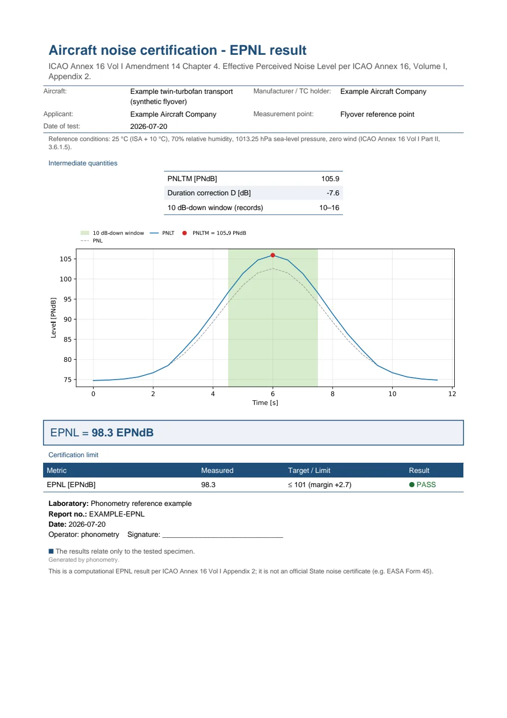
One-page aircraft-noise-certification fiche: a metadata header, a reference-conditions strip, a metrics table with the peak PNLTM and the duration correction D and the 10 dB-down record window, the full-width PNL/PNLT time-history plot with the marked PNLTM and the shaded integration window, the boxed EPNL = 98.3 EPNdB single-number result and a PASS verdict against a 101 EPNdB certification limit.

Download the report (PDF)

ICAO Annex 16 EPNL certification fiche (EPNLResult.report), EPNL in EPNdB with PNLTM and the duration correction D.

Measurement-system verification (IEC 61265)

verify_aircraft_noise_system checks measured performance against the IEC 61265:1995 tolerances: the microphone directional-response limits (Table 1) and the scalar frequency-response, linearity and resolution limits. The one-third-octave filtering is covered by the library’s IEC 61260 class-2 filter verification.

from phonometry import metrology

report = metrology.verify_aircraft_noise_system(
    directional={4000.0: {30: 0.4, 60: 0.9, 90: 1.9, 120: 2.4, 150: 2.4}},
    frequency_response={1000.0: 1.2},
)
print(report["passed"], report["checks"])

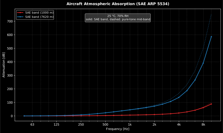
Atmospheric absorption (SAE ARP 5534)

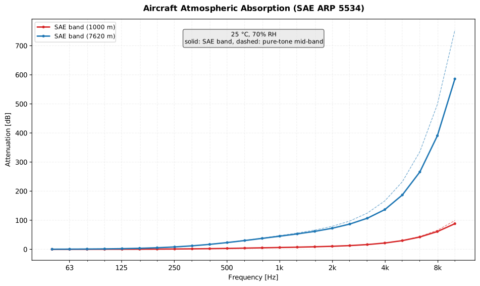
Correcting a measured flyover to reference atmospheric conditions needs the one-third-octave-band attenuation over the path. The pure-tone coefficient is the ISO 9613-1 one (identical, per ARP 5534 §3.1) provided by air_attenuation; sae_band_attenuation adds the SAE Method (ARP 5534 §3.2.2) mapping the pure-tone mid-band path attenuation δ_t = α·s to the band attenuation δ_B, consistent with the Exact Method well beyond the 50 dB Approximate-Method limit.

Show the code for this figure

import matplotlib.pyplot as plt
import numpy as np
from phonometry import aircraft

freqs = 1000.0 * 10.0 ** (np.arange(-13, 11) / 10.0)   # 50 Hz-10 kHz thirds
fig, ax = plt.subplots()
# solid: SAE band attenuation, dashed: pure-tone mid-band
for s in (1000.0, 7620.0):
    att = aircraft.sae_band_attenuation(freqs, s, temperature=25.0, relative_humidity=70.0)
    line, = ax.semilogx(att.frequency, att.band_attenuation, marker="o",
                        markersize=3, label=f"SAE band ({s:.0f} m)")
    ax.semilogx(att.frequency, att.midband_attenuation, "--", alpha=0.6,
                color=line.get_color())
ax.set(xlabel="Frequency [Hz]", ylabel="Attenuation [dB]",
       title="Aircraft atmospheric absorption at 25 °C, 70% RH")
ax.grid(True, which="both", alpha=0.3)
ax.legend()
plt.show()

import numpy as np
from phonometry import aircraft

freqs = 1000.0 * 10.0 ** (np.arange(-13, 11) / 10.0)   # 50 Hz–10 kHz thirds
att = aircraft.sae_band_attenuation(freqs, path_length=7620.0,
                              temperature=25.0, relative_humidity=70.0)
att.plot()   # band vs pure-tone mid-band (needs matplotlib)

Valid roughly 6–32 °C, 20–95 % RH (14 CFR Part 36 window), to 7620 m, reciprocal.

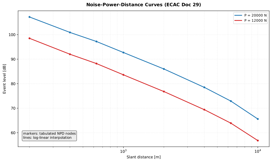
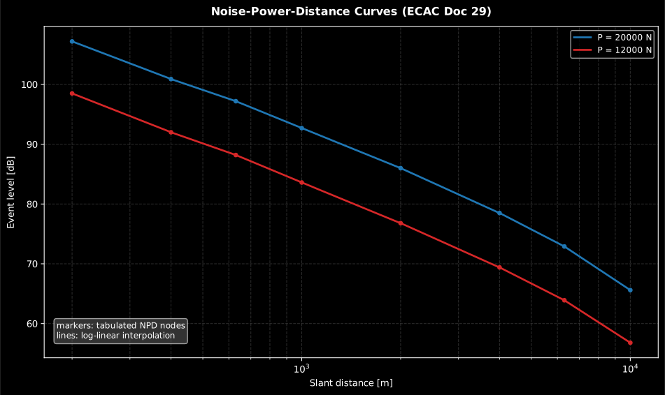
Airport noise: the NPD engine (ECAC Doc 29)

The ECAC Doc 29 airport-noise method describes an aircraft with noise-power- distance (NPD) tables. npd_level reads the event level (LAmax/SEL) for an arbitrary power and distance, interpolating linearly in power (Eq. 4-3) and log-linearly in slant distance (Eq. 4-4).

Show the code for this figure

import matplotlib.pyplot as plt
from phonometry import aircraft

# A schematic NPD table: SEL vs slant distance for two thrust settings.
powers = [12000.0, 20000.0]
distances = [200.0, 400.0, 630.0, 1000.0, 2000.0, 4000.0, 6300.0, 10000.0]
levels = [[98.5, 92.0, 88.2, 83.6, 76.8, 69.4, 63.9, 56.8],
          [107.2, 100.9, 97.2, 92.7, 86.0, 78.5, 72.9, 65.6]]

fig, ax = plt.subplots()
for p in (20000.0, 12000.0):
    curve = aircraft.npd_curve(powers, distances, levels, power=p)
    line, = ax.semilogx(curve.distance, curve.level, label=f"P = {p:.0f} N")
    ax.semilogx(curve.table_distances, curve.table_levels, "o", markersize=4,
                color=line.get_color())
ax.set(xlabel="Slant distance [m]", ylabel="Event level [dB]",
       title="Noise-power-distance curves (ECAC Doc 29)")
ax.grid(True, which="both", alpha=0.3)
ax.legend()
plt.show()

from phonometry import aircraft

powers = [12000.0, 20000.0]
distances = [200.0, 400.0, 1000.0, 2000.0, 6300.0, 10000.0]
levels = [[98.5, 92.0, 83.6, 76.8, 63.9, 56.8],
          [107.2, 100.9, 92.7, 86.0, 72.9, 65.6]]
aircraft.npd_curve(powers, distances, levels, power=20000.0).plot()

This is the NPD engine underneath the method.

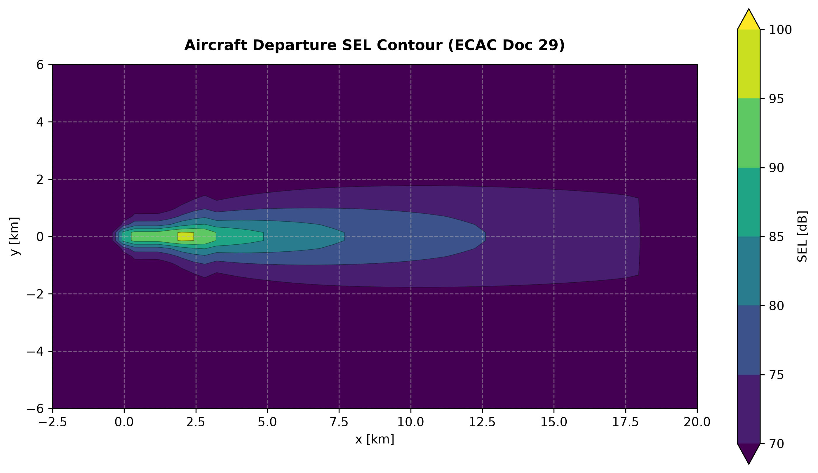
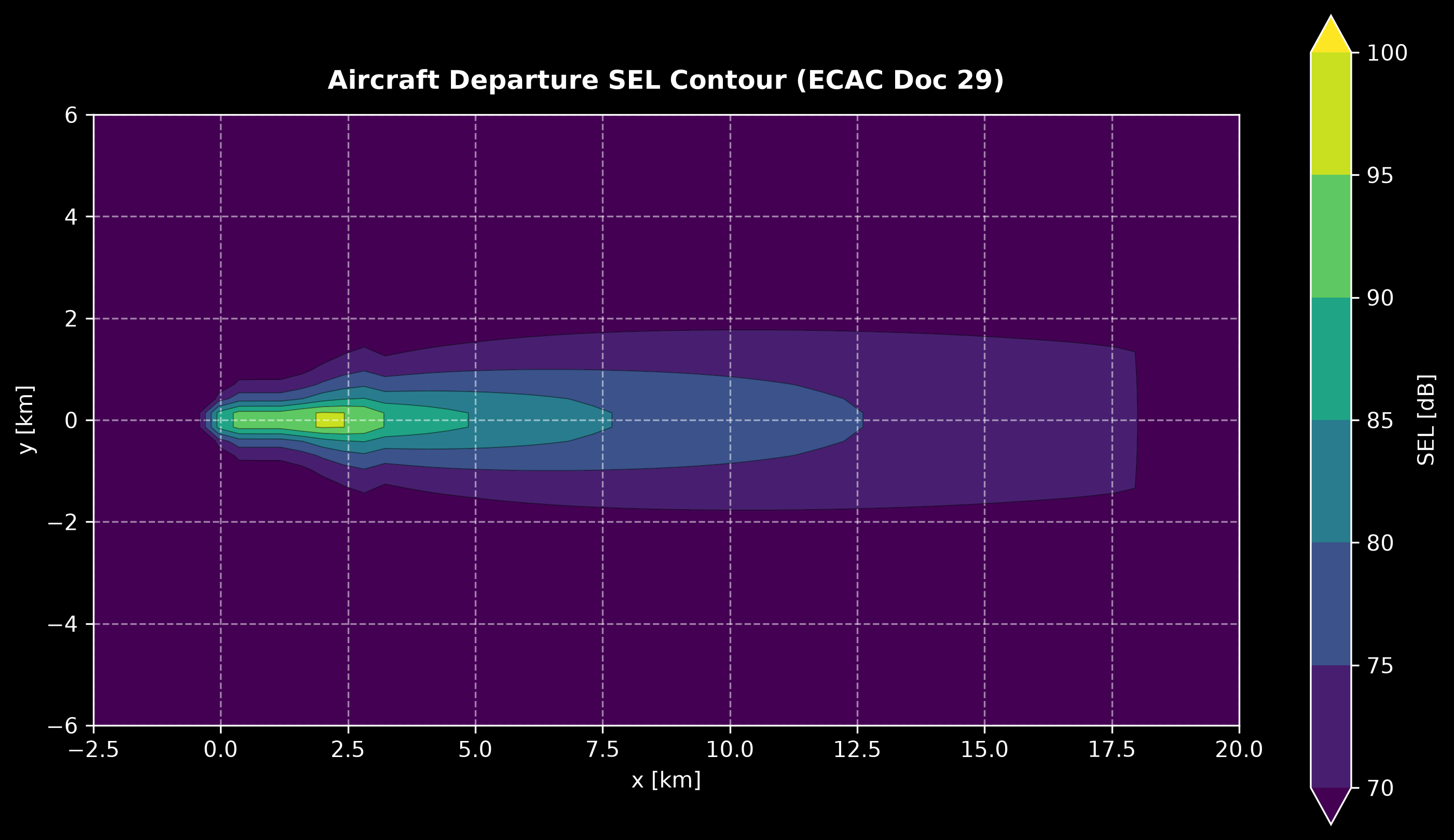
Airport noise contours (single event)

The full single-event calculation breaks a flight path into segments and corrects the NPD baseline per segment (§4.3-4.5): impedance_adjustment (T, p), lateral_attenuation (β,ℓ), engine_installation_correction (φ, mounting), duration_correction, the finite-segment noise_fraction and, behind takeoff ground-roll segments, start_of_roll_directivity (ΔSOR). event_level assembles and sums them into SEL/LAmax, and noise_contour evaluates it over a ground grid (mark the ground-roll segments with a ground_roll mask).

Show the code for this figure

import matplotlib.pyplot as plt
import numpy as np
from phonometry import aircraft

# NPD tables (SEL and LAmax) for one aircraft, two power settings.
powers = [8000.0, 12000.0]
distances = [60.0, 120.0, 240.0, 480.0, 960.0, 1920.0, 3840.0, 7680.0]
sel = [[98.0, 92.0, 86.0, 80.0, 74.0, 68.0, 62.0, 56.0],
       [104.0, 98.0, 92.0, 86.0, 80.0, 74.0, 68.0, 62.0]]
lmax = [[94.0, 88.0, 82.0, 76.0, 70.0, 64.0, 58.0, 52.0],
        [100.0, 94.0, 88.0, 82.0, 76.0, 70.0, 64.0, 58.0]]

# Departure: ground roll along +x, then a steady climb.
xs = np.linspace(0.0, 18000.0, 40)
z = np.clip((xs - 1500.0) * 0.11, 0.0, 2500.0)
power = np.where(xs < 3000.0, 12000.0, 10000.0)
path = np.column_stack([xs, np.zeros_like(xs), z, power, np.full_like(xs, 82.3)])

contour = aircraft.noise_contour(path, powers, distances, sel, lmax,
                                 x=np.linspace(-2500.0, 20000.0, 56),
                                 y=np.linspace(-6000.0, 6000.0, 44))
contour.plot()   # single-event SEL footprint (needs matplotlib)
plt.show()

The mechanism behind these ground corrections is two-path interference: the direct wave and its ground reflection. Below, a 400 Hz source 1.5 m above a rigid plane forms the lobe pattern, with the image source ghosted below the ground and a receiver sitting in an interference dip.

A 2D FDTD simulation of a 400 Hz point source 1.5 metres above rigid ground. The direct and ground-reflected wavefronts interfere and a lobe pattern forms, the ghosted image source below the ground explains the geometry, and the level sampled on an 8 metre arc converges to the two-path image-source model with its predicted nulls.

Download the animation (WebM)

A 2D FDTD simulation of a 400 Hz point source 1.5 metres above rigid ground. The direct and ground-reflected wavefronts interfere and a lobe pattern forms, the ghosted image source below the ground explains the geometry, and the level sampled on an 8 metre arc converges to the two-path image-source model with its predicted nulls.

Download the animation (WebM)

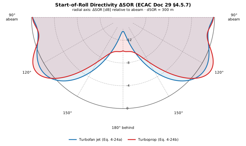
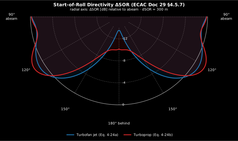
The start-of-roll directivity is the lobed rearward radiation of jet-exhaust noise: strongest near an azimuth ψ ≈ 120° from the nose, falling off abeam (ψ = 90°) and directly behind (ψ = 180°).

Show the code for this figure

import matplotlib.pyplot as plt
import numpy as np
from phonometry import aircraft

az = np.linspace(90.0, 270.0, 361)              # rearward semicircle
psi = np.where(az <= 180.0, az, 360.0 - az)     # ΔSOR is left/right symmetric
jet = [aircraft.start_of_roll_directivity(p, 300.0, "jet") for p in psi]
prop = [aircraft.start_of_roll_directivity(p, 300.0, "turboprop") for p in psi]

ax = plt.subplot(projection="polar")
ax.set_theta_zero_location("N")                 # nose up, azimuth clockwise
ax.set_theta_direction(-1)
ax.plot(np.radians(az), jet, label="Turbofan jet")
ax.plot(np.radians(az), prop, label="Turboprop")
ax.set_rlim(-16.0, 0.0)                         # radial axis: dB re abeam
ax.legend(loc="lower center")
plt.show()

import numpy as np
from phonometry import aircraft

powers = [8000.0, 12000.0]; distances = [60.0, 240.0, 960.0, 3840.0]
sel = [[98.0, 86.0, 74.0, 62.0], [104.0, 92.0, 80.0, 68.0]]
lmax = [[94.0, 82.0, 70.0, 58.0], [100.0, 88.0, 76.0, 64.0]]
xs = np.linspace(0.0, 18000.0, 40)
path = np.column_stack([xs, np.zeros_like(xs), np.clip((xs-1500)*0.11, 0, 2500),
                        np.where(xs < 3000, 12000.0, 10000.0), np.full_like(xs, 82.3)])
aircraft.noise_contour(path, powers, distances, sel, lmax,
                 x=np.linspace(-2500, 20000, 60), y=np.linspace(-6000, 6000, 48)).plot()

Validated against the ECAC Doc 29 5th ed. Vol 3 Part 1 reference workbook: the segment geometry, lateral attenuation, engine installation, noise fraction and the start-of-roll directivity (turbofan and turboprop) reproduce the reference values to < 0.01 dB, and the segment energy sum matches the reference SEL.

The model also covers the landing rollout (landing_roll mask: reduced noise fraction Eq. 4-21b, nearest-end geometry, no directivity term), per-segment bank angle (bank, positive with the starboard wing up; the depression angle is φ = β + ε for observers to starboard of the track and φ = β − ε for observers to port, §4.5.2), the §4.5.5 nearest-end lateral geometry behind takeoff roll, the Eq. 4-13b average runway-segment speed and the recommended 30 m floor on NPD lookups. Seven branch-covering receptor events of the reference workbook are reproduced end-to-end in the test suite.

What this guide covers

Covered. ICAO Annex 16, Vol. I, Appendix 2: perceived noisiness and PNL from Table A2-3 (perceived_noisiness, perceived_noise_level), the slope- method tone correction (tone_correction, matching the ETM Vol. I Table 3-7 turbofan example) and the full EPNL chain (effective_perceived_noise_level, matching the ETM Vol. I Table 4-4 example). IEC 61265:1995 measurement-system tolerances via verify_aircraft_noise_system. SAE ARP 5534 band atmospheric absorption via sae_band_attenuation. The ECAC Doc 29 single-event airport-noise chain (npd_curve, event_level, noise_contour), validated to under 0.01 dB against the Doc 29 5th ed. Vol. 3 Part 1 reference workbook.

Not covered. verify_aircraft_noise_system checks the IEC 61265:1995 tolerances, not the superseding 2018 edition. The airport-noise chain builds single-event contours only: it does not assemble the cumulative multi-event indices (an Lden-style sum over a full flight schedule) that a full Doc 29 noise-contour study needs on top of these single-event levels.

See also

• API reference: aircraft.aircraft_noise, aircraft.airport_noise and aircraft.atmospheric_absorption.

References

• European Civil Aviation Conference. (2016). Report on standard method of computing noise contours around civil airports, Volume 2: Technical guide (ECAC.CEAC Doc 29, 4th ed.). The NPD event-level interpolation (section 4.2) and the single-event segment calculation (impedance adjustment, duration, engine installation, lateral attenuation, noise fraction, start-of-roll directivity, summation) behind the airport noise sections, up to the ground-grid noise contours. The linked PDF is the free download; the volumes are catalogued on the ECAC documents page (https://www.ecac-ceac.org/documents/ecac-documents-and-international-agreements).
• European Civil Aviation Conference. (2026). Report on standard method of computing noise contours around civil airports, Volume 3: Reference cases and verification framework (ECAC.CEAC Doc 29, 5th ed.). The Part 1 reference workbook the single-event chain is validated against. The linked PDF is the free download; the volumes are catalogued on the ECAC documents page (https://www.ecac-ceac.org/documents/ecac-documents-and-international-agreements).
• International Civil Aviation Organization. (2017). Annex 16 to the Convention on International Civil Aviation: Environmental protection — Volume I: Aircraft noise (ICAO Annex 16, Vol. I, 8th ed.). The normative Appendix 2 EPNL procedure implemented by the noisiness, tone correction and EPNL sections.
• International Civil Aviation Organization. (2018). Environmental technical manual — Volume I: Procedures for the noise certification of aircraft (Doc 9501, 3rd ed.). The worked examples (Table 3-7 tone correction, Table 4-4 integrated-method EPNL) used as the numeric oracles.
• International Electrotechnical Commission. (1995). Electroacoustics — Instruments for measurement of aircraft noise — Performance requirements for systems to measure one-third-octave-band sound pressure levels in noise certification of transport-category aeroplanes (IEC 61265:1995). The measurement-system tolerances checked by the verifier. Since revised as IEC 61265:2018 (https://webstore.iec.ch/en/publication/32635); the 1995 edition is the implemented one.
• SAE International. (2006). Method for predicting lateral attenuation of airplane noise (SAE AIR 5662). The soft-ground lateral-attenuation model that Doc 29 adopts (section 4.5.4) in the single-event contour section.
• SAE International. (2012). Standard values of atmospheric absorption as a function of temperature and humidity (SAE ARP 866B, stabilized 2012). The predecessor SAE atmospheric-absorption practice, source of the 50 dB-limited Approximate Method the SAE Method is contrasted with.
• SAE International. (2013). Application of pure-tone atmospheric absorption losses to one-third octave-band data (SAE ARP 5534, reaffirmed 2021). The SAE-Method band attenuation of the atmospheric-absorption section, with the pure-tone coefficient from ISO 9613-1.