Filter Banks

phonometry supports several filter types, each with its own transfer function characteristic. All banks place their −3 dB points on the ANSI S1.11 band edges, so band levels are comparable across architectures.

1. Fractional octave bands: the math

IEC 61260-1:2014 builds every band from the base-10 octave ratio $G=10^{3/10}\approx 1.99526$ (so “one octave” is not exactly 2). For band fraction $1/b$, the mid frequencies and band edges follow (5.2-5.5):

$$f_m=1000\cdot G^{x/b}(b\text{odd}),f_1=f_m{G}^{-1/2b},f_2=f_m{G}^{+1/2b}$$

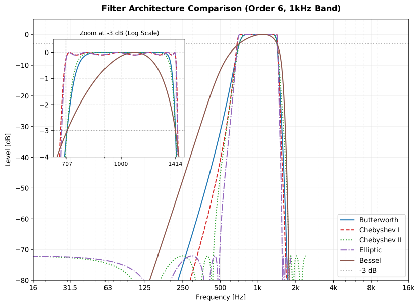
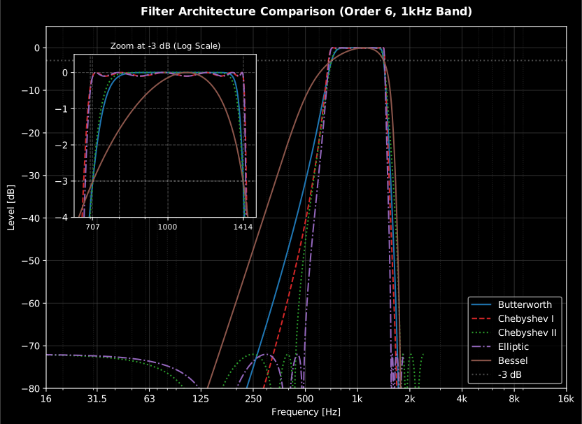
so every 1/3-octave band spans $G^{1/3}\approx 1.2589\approx 10^{1/10}$: ten bands per decade, which is why the nominal frequencies (25, 31.5, 40 …) repeat scaled by 10. phonometry designs each band as an SOS cascade whose −3 dB points land exactly on $f_1$ and $f_2$ for every architecture; for Chebyshev II, Elliptic and Bessel that requires pre-warping the analytic band-edge mapping rather than trusting SciPy’s default parametrization.

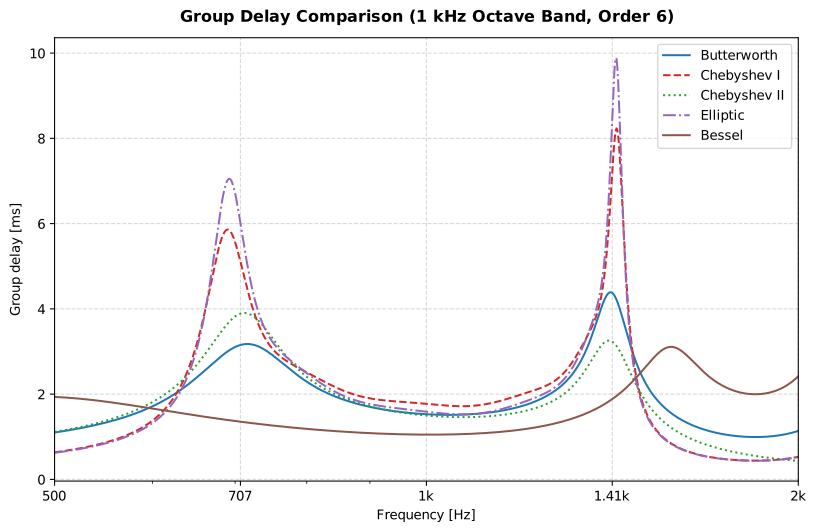
Poles, zeros and stability

A digital band-pass filter is a constellation of poles and zeros in the z-plane: zeros at or near DC and Nyquist pin the response down far from the band (to the stopband floor, for equiripple designs), and the poles cluster just inside the unit circle at the angles $\omega =2\pi f/f_s$ the passband spans. Two intuitions follow. First, selectivity is proximity: the closer the poles sit to the unit circle, the sharper the band and the longer the filter rings (the group-delay peaks of section 8 are that ringing, measured). Second, stability is a margin, not a property of the architecture: an IIR filter is stable only while every pole stays strictly inside the unit circle, and a narrow band at a high sample rate pushes the poles outward (pole radius $\approx 1-\pi B/f_s$ for bandwidth $B$) and squeezes them together, until double-precision coefficients can no longer represent their positions accurately. Second-order sections (SOS) defuse half of the problem: each pole pair keeps its own coefficients, so rounding errors stay local instead of compounding through one high-order polynomial. The other half, the tiny $B/f_s$ ratio itself, is what decimation fixes.

Multirate decimation

A 25 Hz one-third-octave band at 48 kHz spans about 5.8 Hz, 0.024 % of Nyquist, with coefficients so stiff they go numerically unstable. The bank avoids that by filtering low bands at a decimated rate:

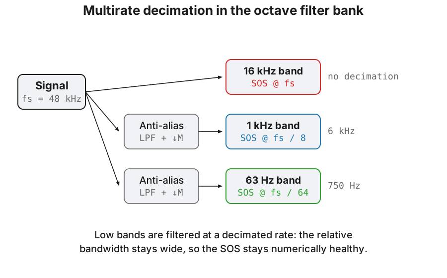
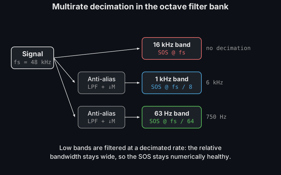
Decimating by $M$ rescales the problem: the same 5.8 Hz bandwidth becomes $M$ times larger relative to the new Nyquist, the pole radius pulls away from the unit circle, and the SOS coefficients return to a well-conditioned range. The price is bookkeeping the bank pays internally: an anti-alias low-pass must run before every decimation stage, because a component above the new Nyquist that folds down lands inside the low bands being measured, and no later filter can remove it.

Aliasing pitfalls

The bank protects its own decimation stages, but it can only analyze what the capture chain delivered:

• Fold-down at the ADC. Energy above $f_s/2$ that reaches the converter without an analog anti-alias filter folds into the analysis range and is indistinguishable from real in-band sound. Sound cards filter this internally; custom instrumentation chains may not.
• Cheap resampling. Converting a 44.1 kHz recording to 48 kHz with a low-quality resampler leaves images that bias the highest bands. Use a polyphase resampler (scipy.signal.resample_poly) or, simpler, analyze at the native rate: every phonometry function takes fs directly.
• Bands near Nyquist. A band whose upper edge approaches $f_s/2$ cannot realize its design response: the bilinear transform compresses the frequency axis there (the same effect the weighting filters counter with high_accuracy). Keep the top band edge comfortably below Nyquist or raise fs, and let verify_filter_class report how much margin is left.

2. Filter Comparison and Zoom

We use Second-Order Sections (SOS) for all filters to ensure numerical stability. The following plot compares the architectures focusing on the -3 dB crossover point.

Show the code for this figure

import matplotlib.pyplot as plt
import numpy as np
from scipy.signal import sosfreqz
from phonometry import metrology

fs = 48000
fig, ax = plt.subplots(figsize=(9, 5))
for ftype in ("butter", "cheby1", "cheby2", "ellip", "bessel"):
    # limits picks out the single 1 kHz octave band
    bank = metrology.OctaveFilterBank(fs, fraction=1, order=6, limits=[800, 1200],
                            filter_type=ftype)
    idx = int(np.argmin(np.abs(np.array(bank.freq) - 1000)))
    fsd = fs / bank.factor[idx]           # rate the band actually runs at
    w, h = sosfreqz(bank.sos[idx], worN=16384, fs=fsd)
    ax.semilogx(w, 20 * np.log10(np.abs(h) + 1e-9), label=ftype)
ax.axhline(-3, color="gray", linestyle=":", label="-3 dB")
ax.set(xlim=(100, 8000), ylim=(-80, 5),
       xlabel="Frequency [Hz]", ylabel="Magnitude [dB]")
ax.grid(True, which="both", alpha=0.3)
ax.legend()
plt.show()

Type	Name	Usage Example	Best For
butter	Butterworth	octave_filter(x, fs, filter_type='butter')	General acoustic measurement.
cheby1	Chebyshev I	octave_filter(x, fs, filter_type='cheby1', ripple=0.1)	Sharper roll-off at the cost of ripple.
cheby2	Chebyshev II	octave_filter(x, fs, filter_type='cheby2')	Flat passband with stopband zeros.
ellip	Elliptic	octave_filter(x, fs, filter_type='ellip', ripple=0.1)	Maximum selectivity.
bessel	Bessel	octave_filter(x, fs, filter_type='bessel')	Preserving transient waveform shapes.

3. octave_filter() / OctaveFilterBank parameters

Parameter	Type	Units	Range / default	Notes
x	1D or 2D array	digital units	non-empty	2D is [channels, samples]
fs	int	Hz	> 0
fraction	int	—	default 1; common 3; any b ≥ 1	Bands per octave = b
order	int	—	default 6	SOS order per band
limits	list [lo, hi]	Hz	default [12, 20000]	Analysis range
filter_type	str	—	'butter' (default), 'cheby1', 'cheby2', 'ellip', 'bessel'	See comparison above
ripple / attenuation	float	dB	ripple default 0.1; attenuation default 72.0	Passband ripple / stopband attenuation (cheby/ellip); cheby2 needs attenuation ≥ 70 for class 1, since scipy pins its equiripple floor at exactly this value
show	bool	—	default False	Plot the bank response (needs matplotlib)
sigbands	bool	—	default False	Also return the per-band time signals
mode	str	—	'rms' (default), 'peak', 'sum'	Per-band statistic returned
nominal	bool	—	default False	Return nominal band labels (e.g. 1000) instead of exact centre frequencies
detrend	bool	—	default True	Remove each band’s DC offset before the level (improves low-frequency accuracy)
calibration_factor	float	—	default 1.0	Scales the input to pascals (see the Calibration guide)
dbfs	bool	—	default False	Reference levels to digital full scale instead of 20 µPa
plot_file	str or None	—	default None	Save the bank-response plot to this path
zero_phase	bool	—	default False	Forward-backward filtering (offline)
stateful / steady_ic (class)	bool	—	default False	Streaming state; see Block Processing

verify_filter_class(bank) checks the designed bank against the IEC 61260-1 Table 1 acceptance limits and reports the class (1, 2 or None if outside both) with per-band margins.

4. Gallery of Filter Bank Responses

Full spectral view of the filter banks for Octave (1/1) and 1/3-Octave fractions.

Architecture	1/1 Octave (Fraction=1)	1/3 Octave (Fraction=3)
Butterworth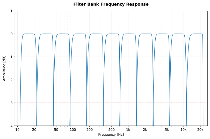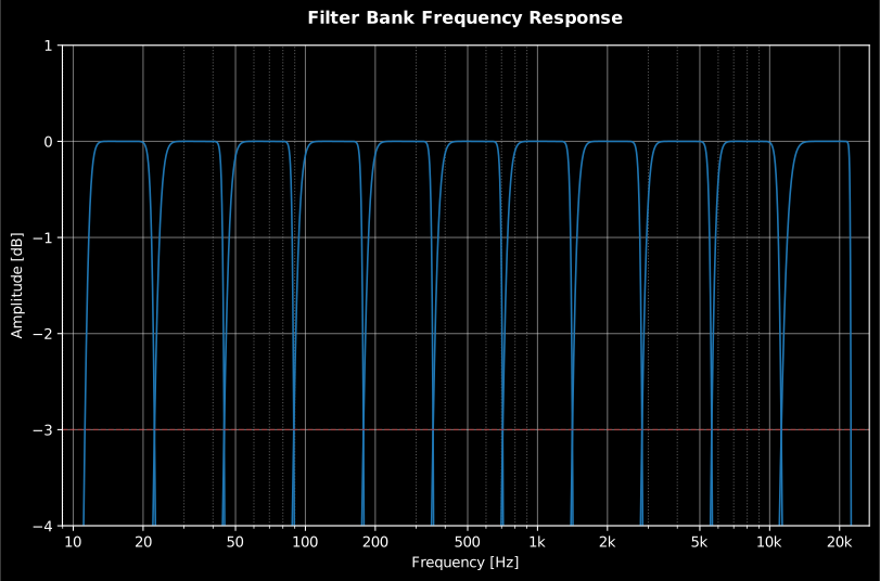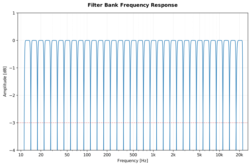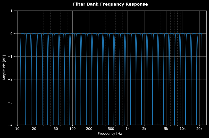
Chebyshev I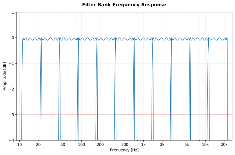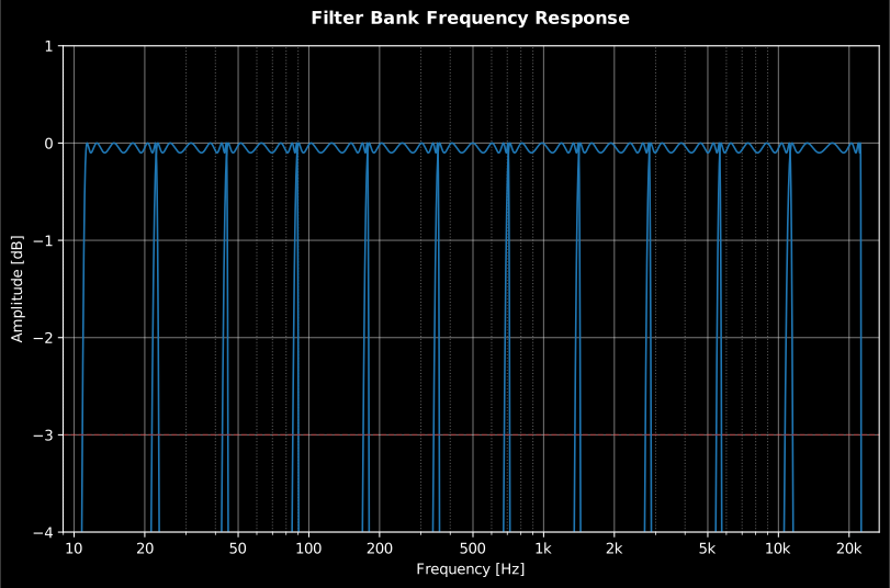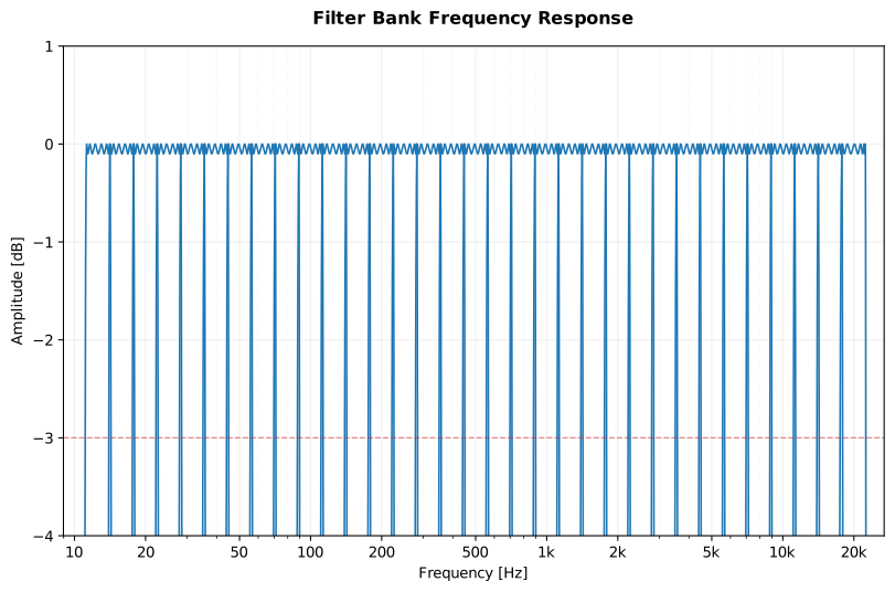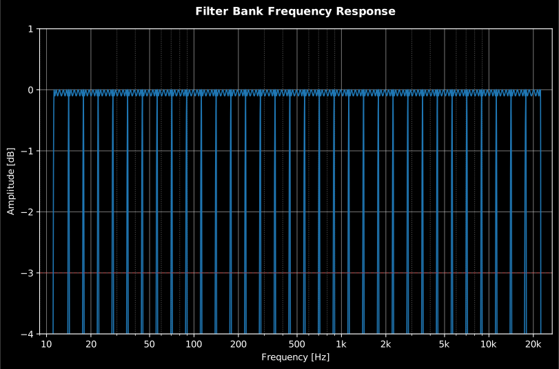
Chebyshev II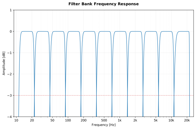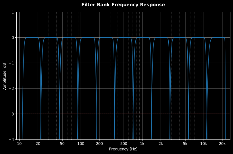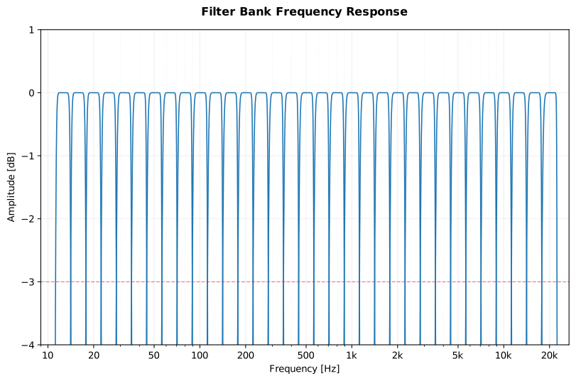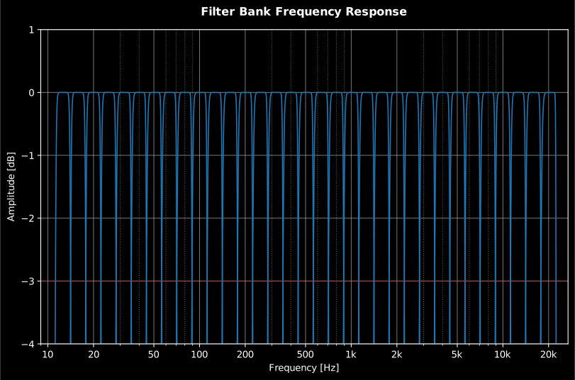
Elliptic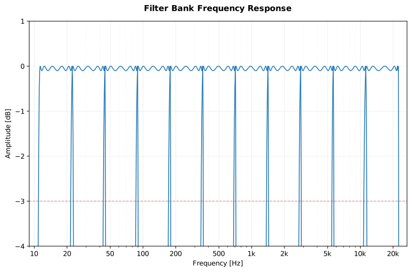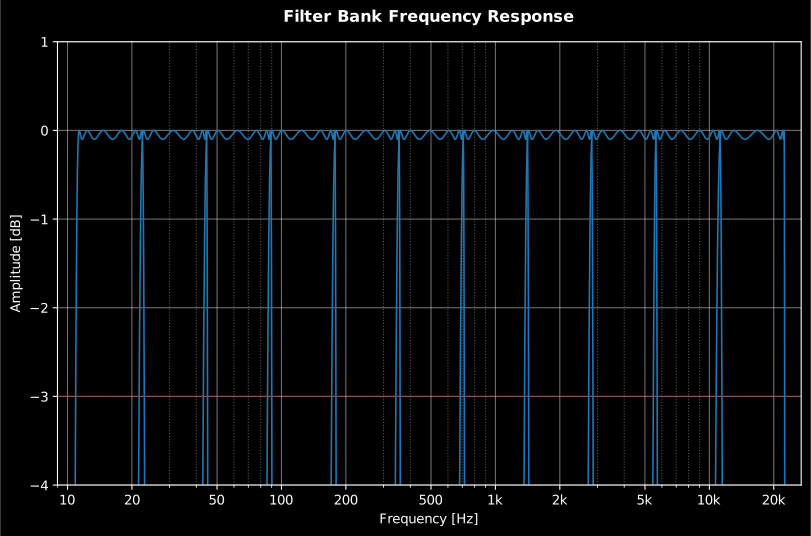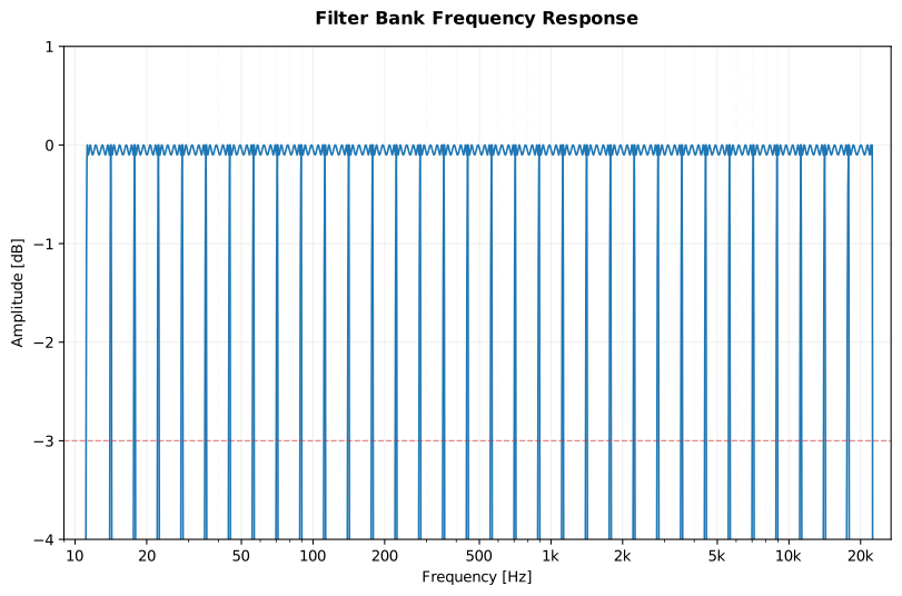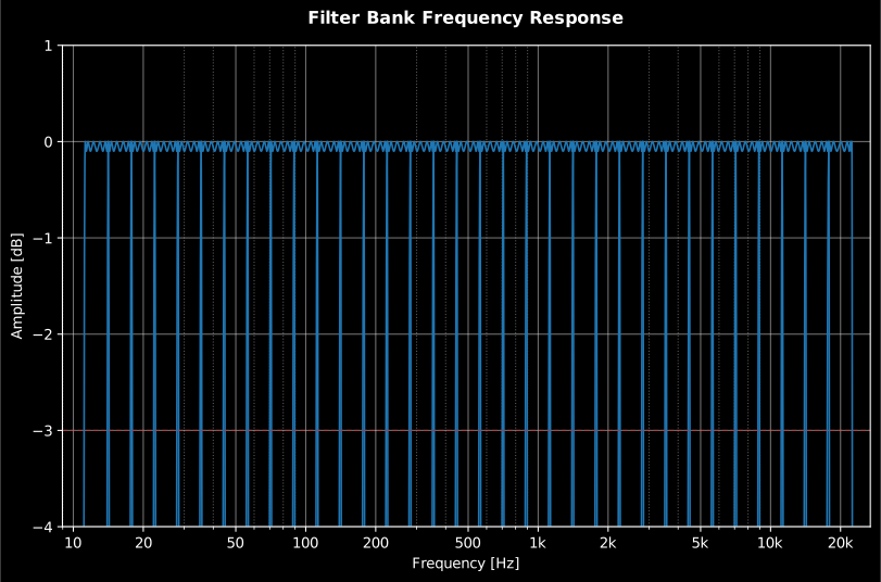
Bessel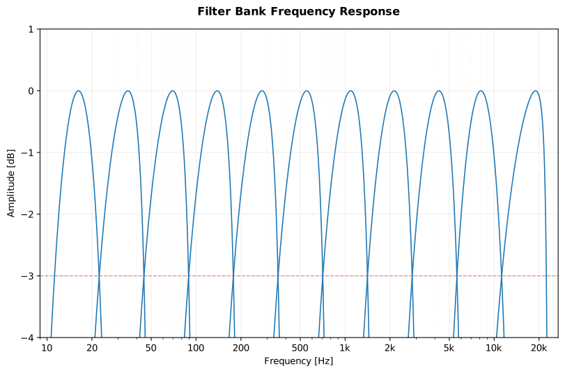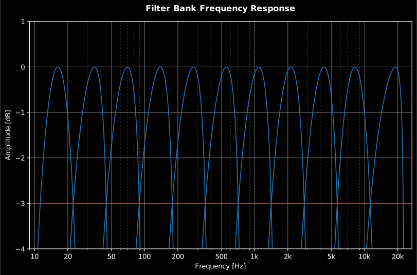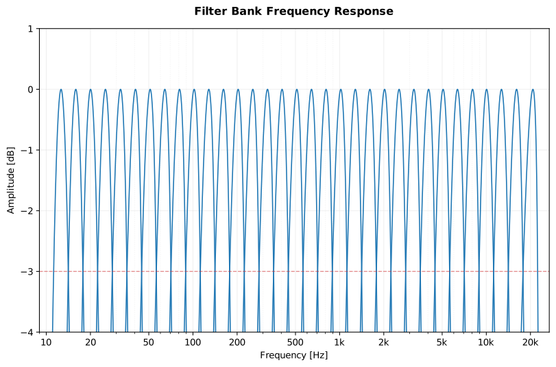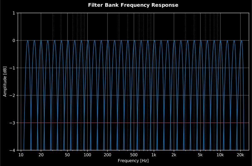

Show the code for this figure

from phonometry import metrology

# One figure per architecture and fraction: the whole response gallery
fs = 48000
for ftype in ("butter", "cheby1", "cheby2", "ellip", "bessel"):
    for fraction in (1, 3):
        # show=True draws the bank's frequency response
        metrology.OctaveFilterBank(fs=fs, fraction=fraction, order=6,
                                   limits=[12, 20000], filter_type=ftype,
                                   show=True)

5. Filter Usage and Examples

1. Butterworth (butter)

The Butterworth filter is known for its maximally flat passband. It is the standard choice for acoustic measurements where no ripple is allowed within the frequency bands.

import numpy as np
from phonometry import metrology

# A calibrated signal in Pa so the guide runs standalone
fs = 48000
x = 0.2 * np.sin(2 * np.pi * 1000 * np.arange(fs) / fs)

# Default standard measurement
spl, freq = metrology.octave_filter(x, fs, filter_type='butter')

Show the code for this figure

from phonometry import metrology

# Draw this bank's response (1/3 octave, order 6, Butterworth)
metrology.OctaveFilterBank(fs=48000, fraction=3, order=6, limits=[12, 20000],
                           filter_type='butter', show=True)

2. Chebyshev I (cheby1)

Chebyshev Type I filters provide a steeper roll-off than Butterworth at the expense of ripples in the passband. Useful when high selectivity is needed near the cut-off frequencies.

import numpy as np
from phonometry import metrology

# A calibrated signal in Pa so the guide runs standalone
fs = 48000
x = 0.2 * np.sin(2 * np.pi * 1000 * np.arange(fs) / fs)

# Selectivity with 0.1 dB passband ripple
spl, freq = metrology.octave_filter(x, fs, filter_type='cheby1', ripple=0.1)

Show the code for this figure

from phonometry import metrology

# Draw this bank's response (1/3 octave, order 6, Chebyshev I)
metrology.OctaveFilterBank(fs=48000, fraction=3, order=6, limits=[12, 20000],
                           filter_type='cheby1', ripple=0.1, show=True)

3. Chebyshev II (cheby2)

Also known as Inverse Chebyshev, it has a flat passband and ripples in the stopband. It provides faster roll-off than Butterworth without affecting the signal in the passband. The stopband edges are placed automatically so that the −3 dB points land on the band edges (attenuation must be > 3.01 dB).

import numpy as np
from phonometry import metrology

# A calibrated signal in Pa so the guide runs standalone
fs = 48000
x = 0.2 * np.sin(2 * np.pi * 1000 * np.arange(fs) / fs)

# Flat passband, class-1 default 72 dB stopband attenuation
spl, freq = metrology.octave_filter(x, fs, filter_type='cheby2')

Show the code for this figure

from phonometry import metrology

# Draw this bank's response (1/3 octave, order 6, Chebyshev II)
metrology.OctaveFilterBank(fs=48000, fraction=3, order=6, limits=[12, 20000],
                           filter_type='cheby2', show=True)

4. Elliptic (ellip)

Elliptic (Cauer) filters have the shortest transition width (steepest roll-off) for a given order. They feature ripples in both the passband and stopband.

import numpy as np
from phonometry import metrology

# A calibrated signal in Pa so the guide runs standalone
fs = 48000
x = 0.2 * np.sin(2 * np.pi * 1000 * np.arange(fs) / fs)

# Maximum selectivity for extreme band isolation
spl, freq = metrology.octave_filter(x, fs, filter_type='ellip', ripple=0.1)

Show the code for this figure

from phonometry import metrology

# Draw this bank's response (1/3 octave, order 6, Elliptic)
metrology.OctaveFilterBank(fs=48000, fraction=3, order=6, limits=[12, 20000],
                           filter_type='ellip', ripple=0.1, show=True)

5. Bessel (bessel)

Bessel filters are optimized for linear phase response and minimal group delay. They preserve the shape of filtered waveforms (transients) better than any other type, but have the slowest roll-off.

import numpy as np
from phonometry import metrology

# A calibrated signal in Pa so the guide runs standalone
fs = 48000
x = 0.2 * np.sin(2 * np.pi * 1000 * np.arange(fs) / fs)

# Best for pulse analysis and transient preservation
spl, freq = metrology.octave_filter(x, fs, filter_type='bessel')

Show the code for this figure

from phonometry import metrology

# Draw this bank's response (1/3 octave, order 6, Bessel)
metrology.OctaveFilterBank(fs=48000, fraction=3, order=6, limits=[12, 20000],
                           filter_type='bessel', show=True)

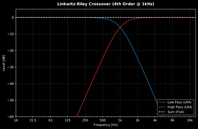
6. Linkwitz-Riley (linkwitz_riley)

Specifically designed for audio crossovers. Linkwitz-Riley filters (typically 4th order, but any even order is supported) allow splitting a signal into bands that, when summed, result in a perfectly flat magnitude response and zero phase difference between bands at the crossover.

import numpy as np
from phonometry import metrology

# recording: a calibrated capture in Pa so the guide runs standalone
fs = 48000
recording = 0.2 * np.sin(2 * np.pi * 1000 * np.arange(fs) / fs)

# Split the recording into Low and High bands at 1000 Hz
low, high = metrology.linkwitz_riley(recording, fs, freq=1000, order=4)
# Reconstruction: low + high == recording (flat response)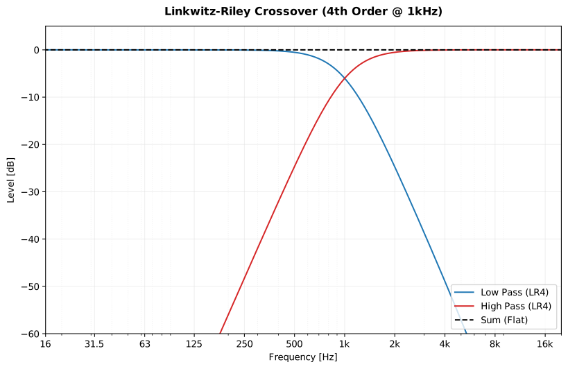

Show the code for this figure

import matplotlib.pyplot as plt
import numpy as np
from scipy.signal import freqz
from phonometry import metrology

# Measure both branches: split a unit impulse and take the spectra.
fs = 48000
impulse = np.zeros(fs)
impulse[0] = 1.0
low, high = metrology.linkwitz_riley(impulse, fs, freq=1000, order=4)

w, h_lp = freqz(low, worN=8192, fs=fs)
_, h_hp = freqz(high, worN=8192, fs=fs)

fig, ax = plt.subplots(figsize=(9, 5))
ax.semilogx(w, 20 * np.log10(np.abs(h_lp) + 1e-9), label="Low-pass (LR4)")
ax.semilogx(w, 20 * np.log10(np.abs(h_hp) + 1e-9), label="High-pass (LR4)")
ax.semilogx(w, 20 * np.log10(np.abs(h_lp + h_hp) + 1e-9), "--",
            label="Sum (flat)")
ax.set(xlim=(20, 20000), ylim=(-60, 5),
       xlabel="Frequency [Hz]", ylabel="Magnitude [dB]")
ax.grid(True, which="both", alpha=0.3)
ax.legend()
plt.show()

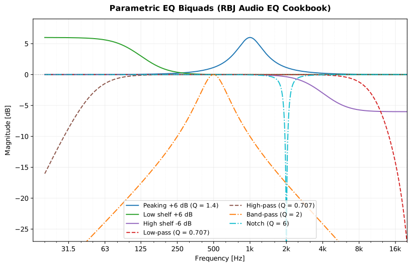
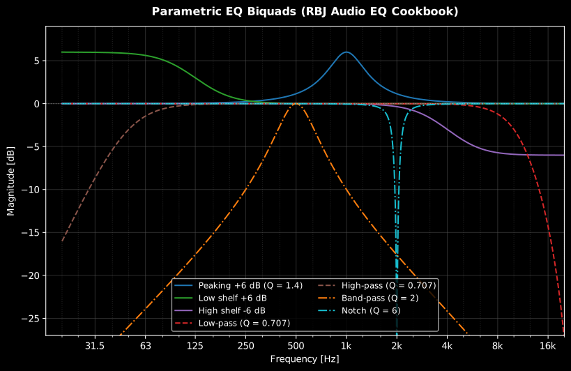
6. Parametric EQ (ParametricEQ)

Biquad equalizer sections per the RBJ Audio EQ Cookbook (Bristow-Johnson): peaking (bell), low/high shelf, low/high-pass, band-pass (constant 0 dB peak or constant skirt gain), notch and all-pass, each parameterized by fs, f0, gain_db and one of q, bw (bandwidth in octaves) or slope exactly as the cookbook defines them. Sections cascade as a numerically robust SOS chain, and the design is closed-form exact: a peaking section passes exactly gain_db at f0 and exactly 0 dB at DC and Nyquist, shelves land exactly on gain_db at their shelved end, and the all-pass has unit magnitude everywhere (only the phase turns).

import numpy as np
from phonometry import EQSection, ParametricEQ

fs = 48000
rng = np.random.default_rng(1)
x = rng.standard_normal(fs)                 # one second of noise

eq = ParametricEQ(fs, [
    EQSection("lowshelf", 100.0, gain_db=4.0),
    EQSection("peaking", 1000.0, gain_db=-6.0, bw=1.0),  # one-octave cut
    EQSection("highshelf", 8000.0, gain_db=3.0),
])
y = eq.filter(x)              # apply the cascade
res = eq.response()           # frozen result carrying the SOS cascade
axes = res.plot()             # magnitude + phase of the cascade

For block processing pass stateful=True (the same convention as WeightingFilter); the one-shot helper is parametric_eq(x, fs, sections).

Show the code for this figure

import matplotlib.pyplot as plt
from phonometry import EQSection, ParametricEQ

fs = 48000
family = [
    EQSection("peaking", 1000.0, gain_db=6.0, q=1.4),
    EQSection("lowshelf", 125.0, gain_db=6.0),
    EQSection("highshelf", 4000.0, gain_db=-6.0),
    EQSection("lowpass", 10000.0),
    EQSection("highpass", 50.0),
    EQSection("bandpass", 500.0, q=2.0),
    EQSection("notch", 2000.0, q=6.0),
]
fig, ax = plt.subplots(figsize=(10, 6))
for section in family:
    res = ParametricEQ(fs, [section]).response(f_min=20.0, f_max=20000.0)
    ax.semilogx(res.frequencies, res.magnitude_db,
                label=f"{section.filter_type} @ {section.f0:g} Hz")
ax.set(xlim=(20, 20000), ylim=(-27, 9),
       xlabel="Frequency [Hz]", ylabel="Magnitude [dB]")
ax.grid(True, which="both", alpha=0.3)
ax.legend(loc="lower center", ncols=2, fontsize=9)
plt.show()

7. Verifying the IEC 61260-1 class

verify_filter_class checks every band of a bank against the acceptance limits of IEC 61260-1:2014 (Table 1, with the fractional-octave breakpoint mapping and log-frequency interpolation from the standard) and reports the performance class per band with its margin in dB:

from phonometry import metrology

bank = metrology.OctaveFilterBank(fs=48000, fraction=3, order=6)
result = metrology.verify_filter_class(bank)
print(result["overall_class"])          # 1
print(result["bands"][0])
# {'freq': 12.589254117941678, 'class': 1, 'margin_class1_db': 0.39999999999997266, 'margin_class2_db': 0.5999999999999727}

The Table 1 acceptance mask itself is public too: class_limits(fraction, filter_class, omega) returns the minimum/maximum relative-attenuation limits at normalized frequencies Ω = f/fm, the same limits the verifier and the figure below use.

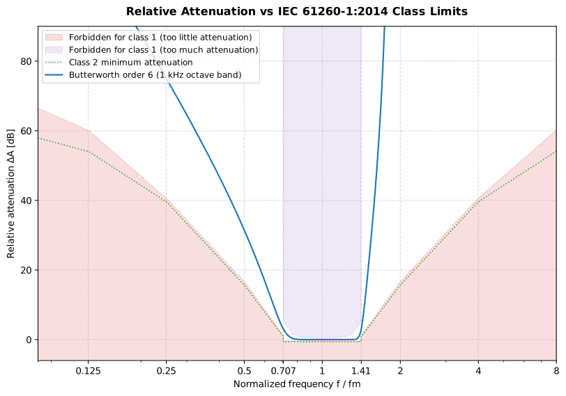
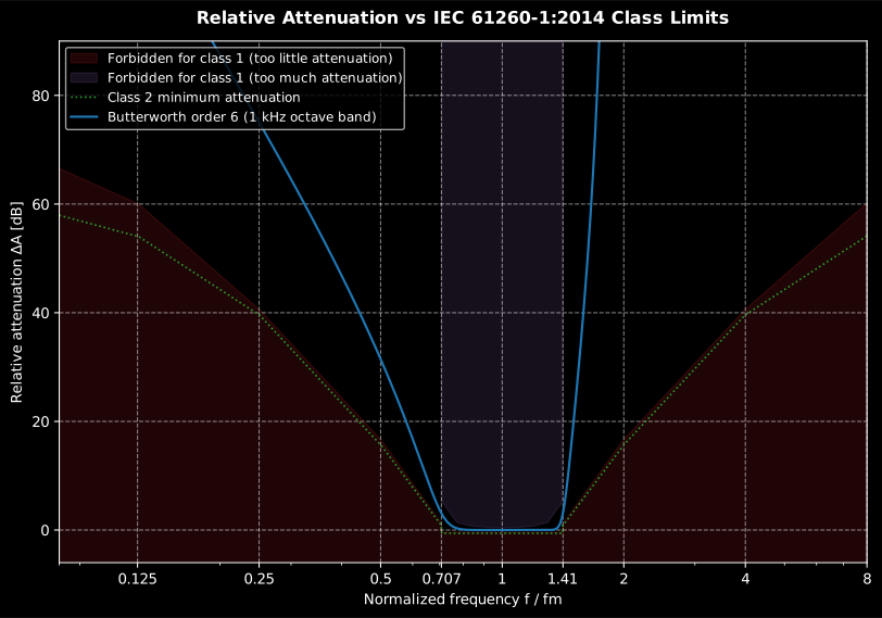
The order-6 Butterworth response (blue) threads between the forbidden regions: it must attenuate at least the red mask outside the band and no more than the purple mask inside it.

Show the code for this figure

import matplotlib.pyplot as plt
import numpy as np
from scipy.signal import sosfreqz
from phonometry import metrology

fs = 48000
bank = metrology.OctaveFilterBank(fs, fraction=1, order=6, limits=[800, 1200])
idx = int(np.argmin(np.abs(np.array(bank.freq) - 1000)))
fm, fsd = bank.freq[idx], fs / bank.factor[idx]
w, h = sosfreqz(bank.sos[idx], worN=2**15, fs=fsd)
att = -20 * np.log10(np.abs(h) + 1e-12)
delta_a = att - np.interp(fm, w, att)     # relative attenuation

grid = np.logspace(np.log10(0.05), np.log10(8), 2000)
lo1, hi1 = metrology.class_limits(1.0, 1, grid)     # class 1 min/max attenuation

fig, ax = plt.subplots(figsize=(9, 5.5))
ax.fill_between(grid, -10, lo1, alpha=0.15, color="tab:red",
                label="Forbidden: too little attenuation")
finite = np.isfinite(hi1)
ax.fill_between(grid[finite], hi1[finite], 90, alpha=0.15, color="tab:purple",
                label="Forbidden: too much attenuation")
ax.plot(w / fm, delta_a, label="Butterworth order 6")
ax.set(xscale="log", xlim=(0.08, 8), ylim=(-6, 90),
       xlabel="Normalized frequency f / fm",
       ylabel="Relative attenuation [dB]")
ax.legend()
plt.show()

With default parameters (order 6), Butterworth meets class 1, and so does Chebyshev II: its attenuation default is now 72 dB, clearing the 70 dB far-stopband class 1 limit (scipy pins the cheby2 equiripple floor at exactly attenuation, so any value ≥ 70 dB qualifies; the 72 dB default keeps the same +0.400 dB passband margin as Butterworth). Chebyshev I, Elliptic and Bessel do not meet class limits at order 6: passband ripple (cheby1/ellip) and slow roll-off (bessel) violate the mask.

Class 0 (IEC 61260:1995 / ANSI S1.11-2004)

The tightest performance class, class 0, was defined by the earlier IEC 61260:1995 and its US twin ANSI S1.11-2004 (both withdrawn/superseded but still referenced for laboratory-grade instruments); IEC 61260-1:2014 dropped it. Its class 1/2 masks differ slightly from the 2014 edition, so it lives behind an edition switch rather than being mixed into the 2014 mask:

from phonometry import metrology

fs = 48000
bank = metrology.OctaveFilterBank(fs, fraction=1, order=6, limits=[800, 1200])

result = metrology.verify_filter_class(bank, edition="1995")   # classes 0, 1, 2
print(result["overall_class"])          # 0  (the default Butterworth clears it)
print(result["bands"][0]["margin_class0_db"])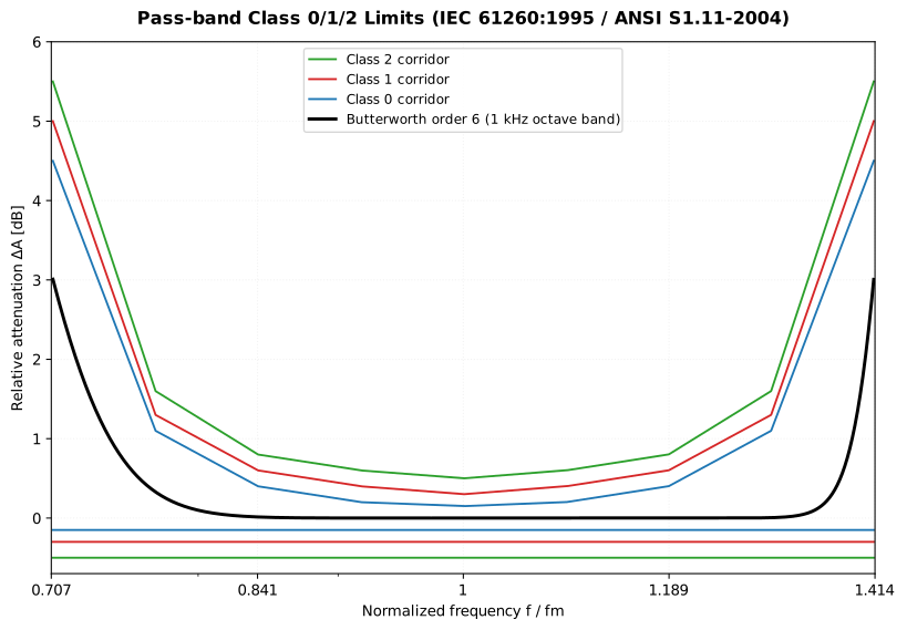

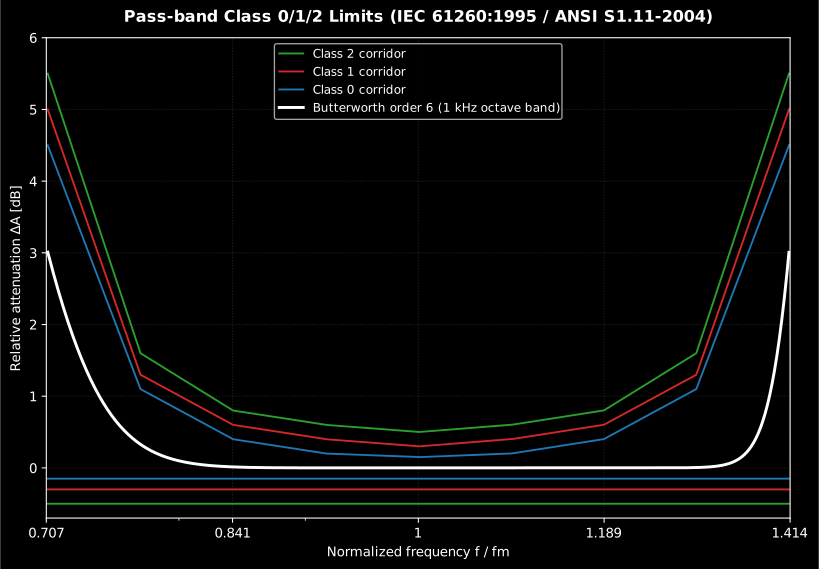
The class 0 corridor (±0.15 dB at mid-band) is the tightest; class 1 (±0.3 dB) and class 2 (±0.5 dB) are progressively wider. The order-6 Butterworth threads inside class 0 across the whole pass-band.

Show the code for this figure

import matplotlib.pyplot as plt
import numpy as np
from scipy.signal import sosfreqz
from phonometry import metrology

fs = 48000
bank = metrology.OctaveFilterBank(fs, fraction=1, order=6, limits=[800, 1200])
idx = int(np.argmin(np.abs(np.array(bank.freq) - 1000)))
fm, fsd = bank.freq[idx], fs / bank.factor[idx]
w, h = sosfreqz(bank.sos[idx], worN=2**15, fs=fsd)
att = -20 * np.log10(np.abs(h) + 1e-12)
delta_a = att - np.interp(fm, w, att)

# Pass-band only: outside the band edges the maximum limit is +inf.
g = 10 ** (3 / 10)
grid = np.linspace(g ** -0.5, g ** 0.5, 1500)
pb = (w / fm >= g ** -0.5) & (w / fm <= g ** 0.5)

fig, ax = plt.subplots(figsize=(9, 5.5))
for cls in (2, 1, 0):                      # nested corridors, class 0 tightest
    lo, hi = metrology.class_limits(1.0, cls, grid, edition="1995")
    ax.plot(grid, hi, label=f"Class {cls} corridor")
    ax.plot(grid, lo, color=ax.lines[-1].get_color())
ax.plot(w[pb] / fm, delta_a[pb], "k", lw=2, label="Butterworth order 6")
ax.set(xscale="log", xlim=(g ** -0.5, g ** 0.5), ylim=(-0.7, 6),
       xlabel="Normalized frequency f / fm",
       ylabel="Relative attenuation [dB]")
ax.legend()
plt.show()

What a class means physically

The masks are worst-case error bounds on a measurement, not abstract grades:

• In the passband the corridor bounds how much the band can mis-read in-band content: a class 1 bank reads a mid-band tone within ±0.4 dB of its true level and a class 2 bank within ±0.6 dB (2014 Table 1; the stricter 1995 masks allowed ±0.3 dB for class 1 and ±0.15 dB for class 0). Toward the band edges the corridor widens, which is the honest admission that a tone sitting exactly on an edge is genuinely ambiguous between two bands (both read it about 3 dB down).
• In the stopband the minimum-attenuation mask bounds leakage from the rest of the spectrum: far from the band, class 1 demands at least 70 dB of relative attenuation (the reason the cheby2 default is 72 dB). In energy terms, an out-of-band tone must be roughly 70 dB stronger than the band’s own content before it doubles the band’s energy reading (+3 dB). The practical consequence: measuring bands far below a dominant tone, the reading floors out at the leakage skirt about 70 dB down, and a steeper architecture (or higher order) is the only way to push that floor lower.
• For the uncertainty budget, the class is the filter’s contribution to the measurement uncertainty: a class 1 bank adds up to a few tenths of a dB to a band level, comparable to a class 1 sound level meter’s other tolerance terms, which is why instrument-grade chains specify the class of every stage rather than a single overall figure.

Which architecture reaches which class? The library’s default, Butterworth order 6, meets class 0 in the configurations the conformance suite verifies (octave and third-octave banks at 48 kHz), so no special setup is needed for laboratory-grade banks in that range. The table below reports the best class each architecture reaches under that same order-6 / 48 kHz setup; the other architectures fall short of class 0 because they trade the IEC mask for a different property by construction:

Architecture	Best class (order 6, fs 48 kHz)	Why
butter (default)	0	Maximally-flat pass-band, monotone roll-off; fits the mask
cheby2	1	Flat pass-band but the mask relationship binds at class 1
cheby1	—	Pass-band ripple violates the flatness limit
ellip	—	Pass- and stop-band ripple
bessel	—	Flat group delay bought with a slow roll-off

So the sensible default is the common one (Butterworth order 6): it clears class 0 in the verified configurations, while the alternative architectures are deliberate opt-ins whose purpose (steeper roll-off, linear phase) works against the class mask. Away from these settings (very high fraction or near-Nyquist bands), always re-run verify_filter_class to confirm the class you need, and raise the order if a band needs more margin.

IEC 61260-1 filter compliance report (.report())

filter_class_compliance(bank) wraps the same verification as a result object that exposes .plot() and .report(), so a type-test verdict can be rendered as a one-page accredited fiche. The fiche lists every band’s achieved class and its binding margin, overlays the worst-margin band’s measured relative attenuation on the class corridor, and boxes the overall class-compliance result. Pass a required_class on the ReportMetadata to add a PASS/FAIL verdict row (a bank “meets class N” when its achieved class is at least as strict, i.e. a class index of N or lower). The fiche renders in English by default; pass language="es" for a Spanish fiche (translated fixed strings and a comma decimal separator), e.g. result.report("iec61260_es.pdf", language="es").

from phonometry import (
    OctaveFilterBank,
    ReportMetadata,
    filter_class_compliance,
)

bank = OctaveFilterBank(fs=48000, fraction=1, order=6, limits=[125, 4000])
result = filter_class_compliance(bank)   # overall_class == 1
result.plot()   # the worst-margin band on its class corridor

result.report(
    "iec61260.pdf",
    metadata=ReportMetadata(
        specimen="1/1-octave filter bank",
        measurement_standard="IEC 61260-1:2014",
        required_class=1,                # class 1 (or stricter) required
    ),
)                                        # -> Class 1 - COMPLIES, PASS

The example fiche is regenerated with make reports and kept rendered in the repository; click the preview to open the PDF.

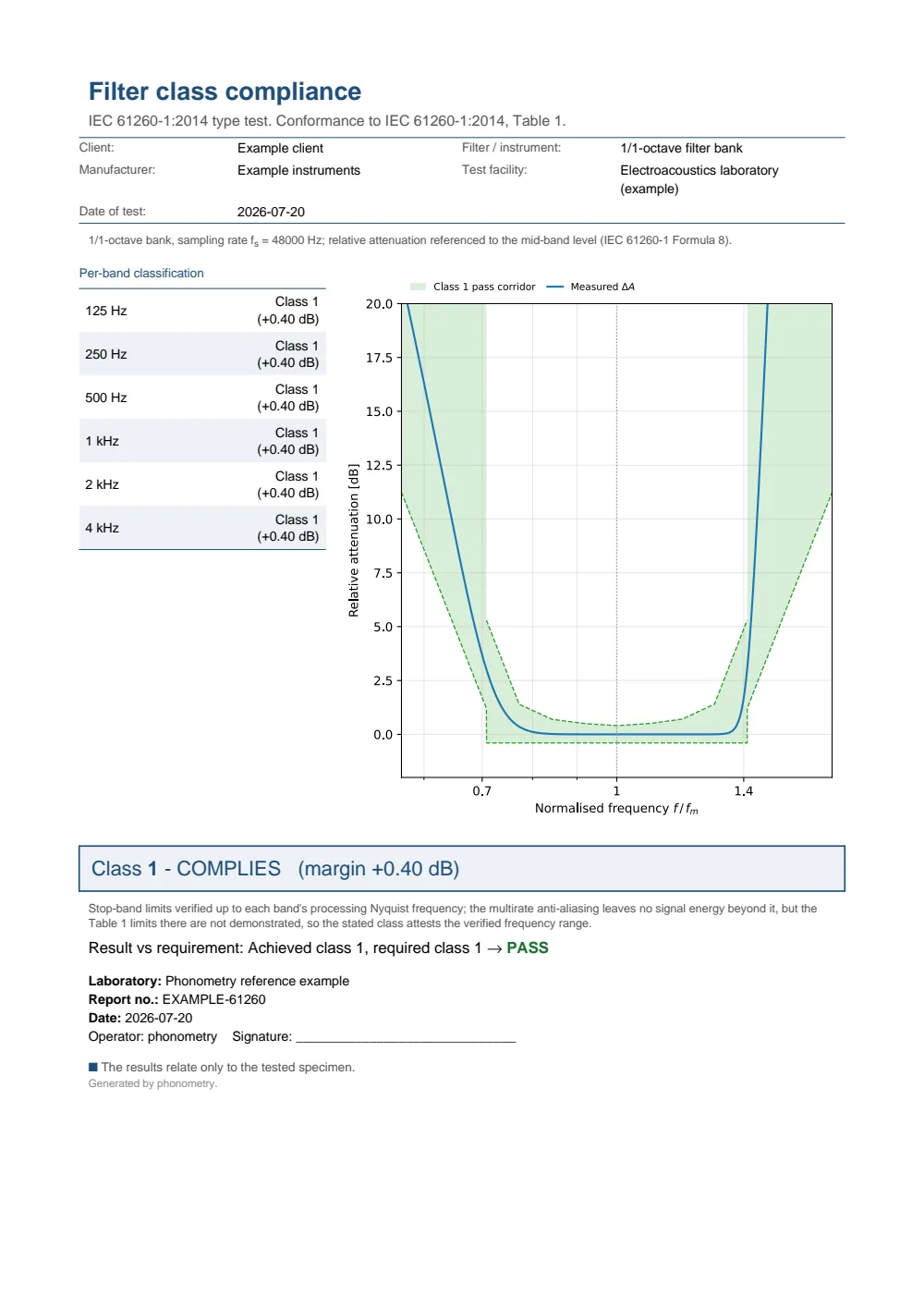
One-page filter-class-compliance fiche: a metadata header, a per-band classification table listing each octave band's achieved class and binding margin, the worst-margin band's measured relative attenuation overlaid on the green class-1 acceptance corridor, the boxed Class 1 - COMPLIES (margin +0.40 dB) result and a PASS verdict against the required class 1.

Download the report (PDF)

Filter class compliance fiche (FilterComplianceResult.report), achieved class with the binding margin in dB and the measured relative attenuation over the Table 1 corridor.

Passing edition="1995" verifies against the older IEC 61260:1995 / ANSI S1.11-2004 mask, which keeps the stricter class 0 that the 2014 edition dropped, so a modest order-6 bank can be certified to class 0:

bank = OctaveFilterBank(fs=48000, fraction=1, order=6, limits=[250, 4000])
result = filter_class_compliance(bank, edition="1995")   # overall_class == 0
result.plot()   # the class-0 corridor of the 1995 edition
result.report("iec61260_1995.pdf",
              metadata=ReportMetadata(measurement_standard="IEC 61260:1995",
                                      required_class=0))   # -> Class 0 - COMPLIES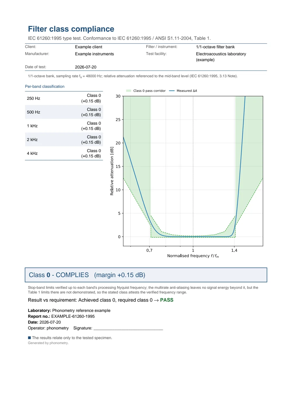

One-page filter-class-compliance fiche under the 1995 edition: a per-band classification table showing every octave band achieving class 0, the measured relative attenuation overlaid on the green class-0 acceptance corridor, the boxed Class 0 - COMPLIES (margin +0.15 dB) result and a PASS verdict against the required class 0.

Download the report (PDF)

Class 0 is retained by the IEC 61260:1995 / ANSI S1.11-2004 edition (edition='1995'); the 2014 edition keeps only classes 1 and 2.

8. Signal Decomposition and Stability

By setting sigbands=True, you can retrieve the time-domain components of each band. This allows for advanced analysis or comparing how different architectures (e.g., Butterworth vs Chebyshev) affect the signal phase and transient response.

import numpy as np
from phonometry import metrology

# 1. Generate a signal (Sum of 250Hz and 1000Hz)
fs = 48000
t = np.linspace(0, 0.5, int(fs * 0.5), endpoint=False)
y = np.sin(2 * np.pi * 250 * t) + np.sin(2 * np.pi * 1000 * t)

# 2. Compare architectures (Butterworth vs Chebyshev II)
spl_b, freq, xb_butter = metrology.octave_filter(y, fs=fs, fraction=1, sigbands=True, filter_type='butter')
spl_c2, _, xb_cheby2 = metrology.octave_filter(y, fs=fs, fraction=1, sigbands=True, filter_type='cheby2')

# 'xb_butter' and 'xb_cheby2' contain the time-domain signals per band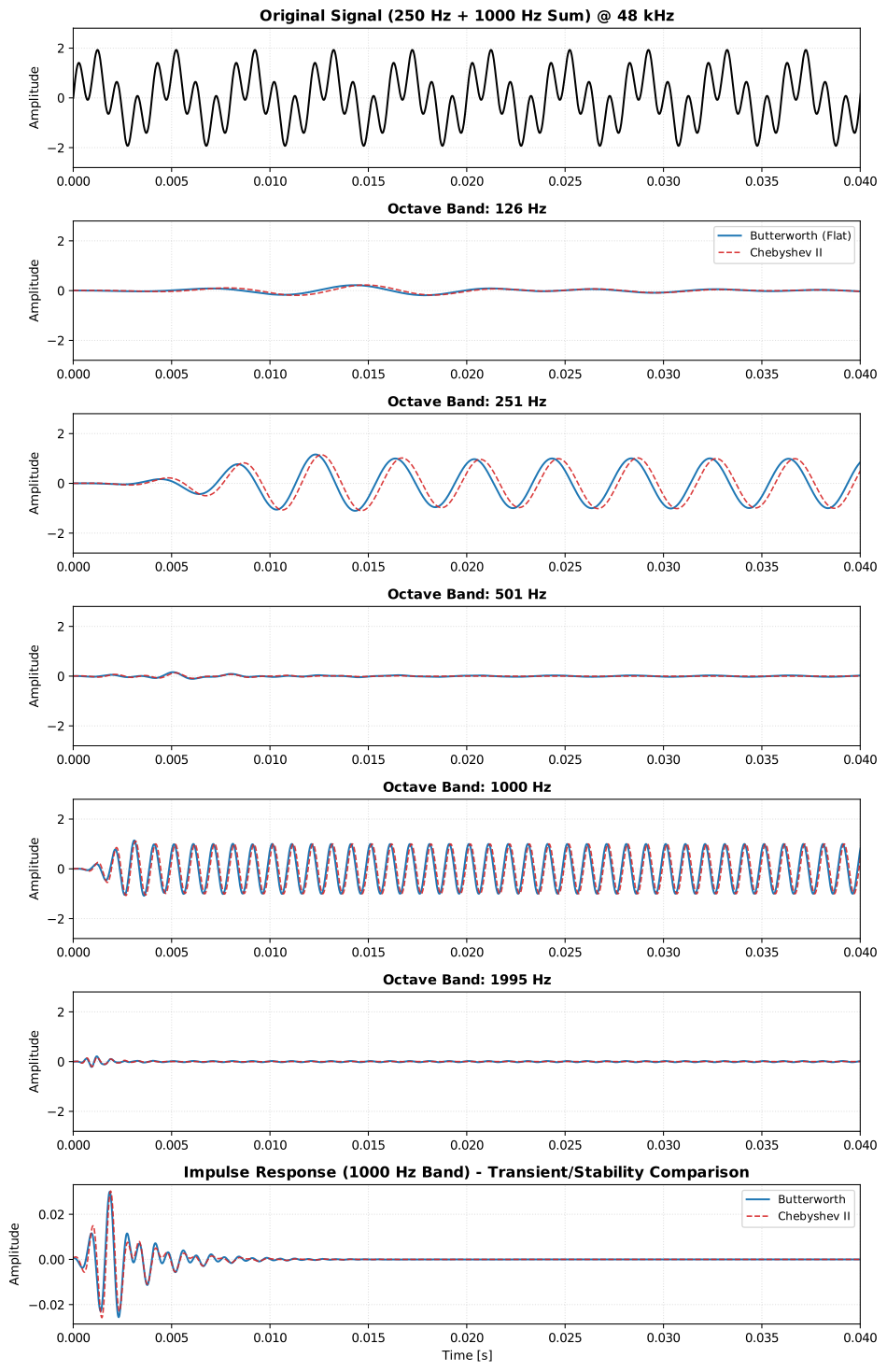

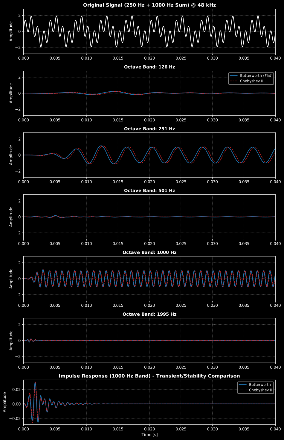
The plot compares the Butterworth (solid blue) and Chebyshev II (dashed red) responses. The bottom plot shows the Impulse Response, highlighting the differences in stability and transient decay.

Show the code for this figure

import matplotlib.pyplot as plt
import numpy as np
from phonometry import metrology

fs = 48000
t = np.linspace(0, 0.5, int(fs * 0.5), endpoint=False)
y = np.sin(2 * np.pi * 250 * t) + np.sin(2 * np.pi * 1000 * t)

bank_b = metrology.OctaveFilterBank(fs=fs, fraction=1, order=6, limits=[100.0, 2000.0])
bank_c = metrology.OctaveFilterBank(fs=fs, fraction=1, order=6, limits=[100.0, 2000.0],
                          filter_type="cheby2")
_, freq, xb_butter = bank_b.filter(y, sigbands=True)
_, _, xb_cheby2 = bank_c.filter(y, sigbands=True)

fig, axes = plt.subplots(len(freq), 1, figsize=(9, 2 * len(freq)), sharex=True)
for ax, fc, xb, xc in zip(axes, freq, xb_butter, xb_cheby2):
    ax.plot(t, xb, label="Butterworth")
    ax.plot(t, xc, "--", label="Chebyshev II")
    ax.set_title(f"{fc:.0f} Hz band")
    ax.set_xlim(0, 0.04)
axes[0].legend()
axes[-1].set_xlabel("Time [s]")
plt.tight_layout()
plt.show()

Note

Why do the signals look shifted in time? Digital IIR filters (like Butterworth or Chebyshev) have non-linear phase responses, which results in frequency-dependent Group Delay. In the 250 Hz band, you can see that the Chebyshev II filter has a different propagation delay compared to the Butterworth filter. This is a normal physical property of these architectures: more aggressive frequency roll-offs usually come at the cost of higher group delay and phase distortion.

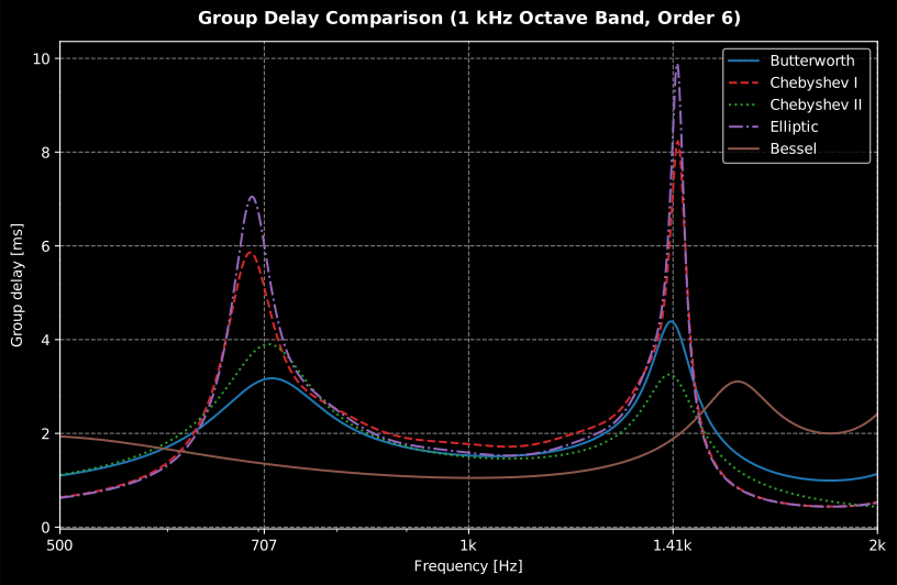
Group delay, quantified

The group delay ${\tau }_g(\omega )=-\frac{d\varphi (\omega )}{d\omega }$ of the 1 kHz octave band shows the trade-off directly: Bessel stays nearly flat across the passband (transient shapes survive), while Chebyshev I and Elliptic pay for their steep roll-off with strong delay peaks at the band edges.

Show the code for this figure

import matplotlib.pyplot as plt
import numpy as np
from scipy.signal import group_delay
from phonometry import metrology

fs = 48000
w = np.logspace(np.log10(500), np.log10(2000), 1024)
fig, ax = plt.subplots(figsize=(9, 5))
for ftype in ("butter", "cheby1", "cheby2", "ellip", "bessel"):
    bank = metrology.OctaveFilterBank(fs, fraction=1, order=6, limits=[800, 1200],
                            filter_type=ftype)
    idx = int(np.argmin(np.abs(np.array(bank.freq) - 1000)))
    fsd = fs / bank.factor[idx]
    # Group delay of an SOS cascade = sum of the sections' group delays
    gd = sum(group_delay((sec[:3], sec[3:]), w=w, fs=fsd)[1]
             for sec in bank.sos[idx])
    ax.semilogx(w, gd / fsd * 1000, label=ftype)
ax.set(xlim=(500, 2000), xlabel="Frequency [Hz]", ylabel="Group delay [ms]")
ax.grid(True, which="both", alpha=0.3)
ax.legend()
plt.show()

9. Zero-phase filtering

For offline analysis you can eliminate group delay entirely: zero_phase=True filters each band forward-backward (scipy.signal.sosfiltfilt), keeping band signals time-aligned with the input. The effective attenuation doubles and the effective passband narrows, lowering the measured broadband band level by ~0.2 to 0.3 dB per band (a pure in-band tone is unaffected); prefer forward filtering when the absolute band SPL must match single-pass conventions, and reserve zero-phase for when the temporal envelope matters (e.g. reverberation decay). The option is incompatible with stateful (block) processing.

import numpy as np
from phonometry import metrology

fs = 48000
t = np.linspace(0, 0.5, int(fs * 0.5), endpoint=False)
y = np.sin(2 * np.pi * 250 * t) + np.sin(2 * np.pi * 1000 * t)

bank = metrology.OctaveFilterBank(fs=48000, fraction=3)
spl, freq, xb = bank.filter(y, sigbands=True, zero_phase=True)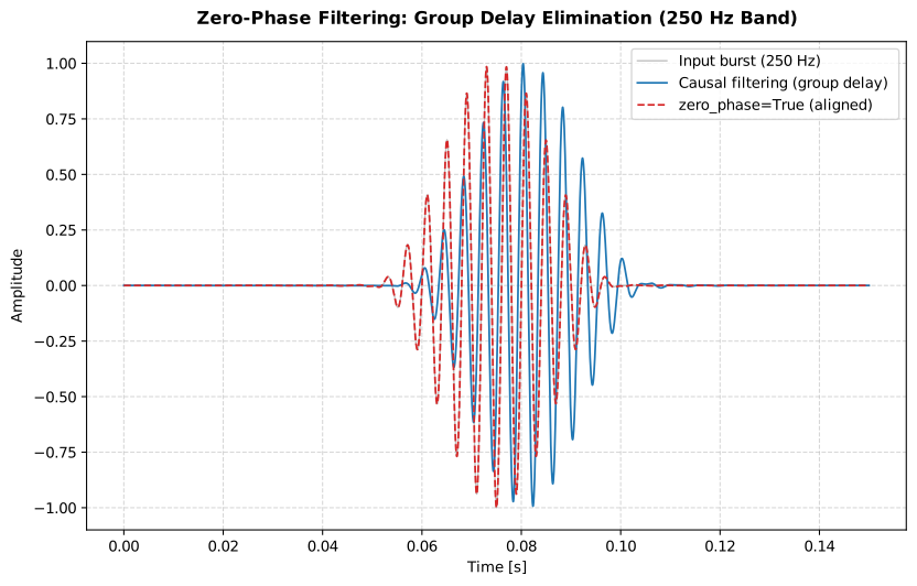

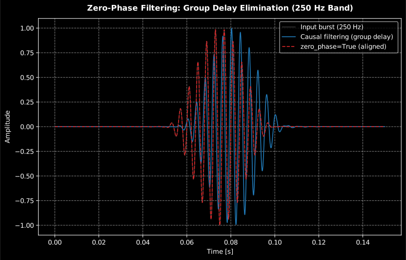
Causal filtering delays the burst by the filter’s group delay; zero-phase filtering keeps it aligned with the input.

Show the code for this figure

import matplotlib.pyplot as plt
import numpy as np
from phonometry import metrology

fs = 48000
t = np.linspace(0, 0.15, int(fs * 0.15), endpoint=False)
x = np.zeros_like(t)                      # 250 Hz tone burst mid-frame
start, end = int(0.05 * fs), int(0.10 * fs)
x[start:end] = np.sin(2 * np.pi * 250 * t[start:end]) * np.hanning(end - start)

bank = metrology.OctaveFilterBank(fs=fs, fraction=1, order=6, limits=[200.0, 300.0])
_, _, fwd = bank.filter(x, sigbands=True, calculate_level=False)
_, _, zp = bank.filter(x, sigbands=True, calculate_level=False,
                       zero_phase=True)

fig, ax = plt.subplots(figsize=(9, 4.5))
ax.plot(t, x, color="gray", alpha=0.5, label="Input burst (250 Hz)")
ax.plot(t, fwd[0], label="Causal (group delay)")
ax.plot(t, zp[0], "--", label="zero_phase=True (aligned)")
ax.set(xlabel="Time [s]", ylabel="Amplitude")
ax.legend()
plt.show()

What this guide covers

Covered. IEC 61260-1:2014’s band-edge mathematics (clauses 5.2-5.5) and Table 1 class 1/2 acceptance limits, verified by verify_filter_class and reported by filter_class_compliance().report(); the withdrawn IEC 61260:1995 / ANSI S1.11-2004 class 0 mask, reachable with edition="1995"; and the ISO 266:1997 preferred-frequency series behind nominal_frequencies. The library designs each band as an SOS cascade across five architectures (Butterworth, Chebyshev I/II, Elliptic, Bessel), plus the Linkwitz-Riley crossover and the RBJ Audio EQ Cookbook’s ParametricEQ.

Not covered. IEC 61260-1’s conformance tests for the physical filter itself (overload recovery, filter linearity, environmental influences) apply to hardware analog and digital filters and are not implemented: verify_filter_class checks the designed digital response against Table 1, not an instrument. Near Nyquist, the bilinear transform warps the frequency axis and the bank has no correction for it (unlike WeightingFilter’s high_accuracy option): keep the top band edge comfortably below Nyquist or raise fs, and confirm the margin with verify_filter_class.

See also

• API reference: phonometry, metrology.core and metrology.parametric_filters.

Quick answers

How are fractional-octave centre frequencies and band edges defined?

IEC 61260-1:2014 (clauses 5.2-5.5) builds every band from the base-10 octave ratio $G=10^{3/10}\approx 1.99526$, so one octave is not exactly 2. Mid frequencies follow $f_m=1000\cdot G^{x/b}$ (for odd $b$) and the edges are $f_1=f_m{G}^{-1/2b}$ and $f_2=f_m{G}^{+1/2b}$; every one-third-octave band spans $G^{1/3}\approx 1.2589$, ten bands per decade.

Which filter architecture meets IEC 61260-1 class 1 with default settings?

With the default order 6, Butterworth meets class 1 of the IEC 61260-1:2014 Table 1 acceptance limits, and so does Chebyshev II: its default attenuation of 72 dB clears the 70 dB far-stopband class 1 limit. Chebyshev I, Elliptic and Bessel do not: passband ripple (cheby1, ellip) and slow roll-off (bessel) violate the mask. verify_filter_class reports the achieved class per band.

What is class 0 and which standard defines it?

Class 0 is the tightest filter performance class, defined by IEC 61260:1995 and its US twin ANSI S1.11-2004 and dropped by IEC 61260-1:2014. Its passband corridor allows only ±0.15 dB at mid-band, against ±0.3 dB for class 1 in the 1995 masks. It stays available through edition="1995", and the default order-6 Butterworth bank meets class 0 in the verified 48 kHz configurations.

References

• American National Standards Institute. (2004). Specification for octave-band and fractional-octave-band analog and digital filters (ANSI S1.11-2004). Acoustical Society of America. Its Table 1 class limits are identical to those of IEC 61260:1995 and back the same class 0 mask.
• Bristow-Johnson, R. (2021). Audio EQ Cookbook. W3C Working Group Note (ed. R. Toy), 8 June 2021. The biquad coefficient recipes and the Q / bandwidth / shelf-slope parameterization behind ParametricEQ (section 6).
• International Electrotechnical Commission. (1995). Electroacoustics — Octave-band and fractional-octave-band filters (IEC 61260:1995). The withdrawn first edition whose Table 1 supplies the stricter class 0 mask offered by edition='1995', and the band-edge convention on which every bank places its −3 dB points.
• International Electrotechnical Commission. (2014). Electroacoustics — Octave-band and fractional-octave-band filters — Part 1: Specifications (IEC 61260-1:2014). The band-edge mathematics of section 1 (base-10 mid frequencies and band edges, clauses 5.2-5.5), the nominal band labels, and the Table 1 class 1/class 2 acceptance limits (with the fractional-octave breakpoint mapping and log-frequency interpolation) verified in section 6.
• International Organization for Standardization. (1997). Acoustics — Preferred frequencies (ISO 266:1997). The preferred-frequency series behind the nominal band labels reported by nominal_frequencies.
• Oppenheim, A. V., & Schafer, R. W. (2010). Discrete-time signal processing (3rd ed.). Pearson. The pole-zero, stability and multirate theory condensed in section 1: SOS cascades, the bilinear transform and decimation (ISBN 978-0-13-198842-2).
• Smith, J. O. (n.d.). Introduction to digital filters with audio applications. Center for Computer Research in Music and Acoustics (CCRMA), Stanford University. A free online-book companion treatment of digital-filter design and analysis, from pole-zero geometry to filter stability.