Atmospheric refraction: rays and the GFPE

The ISO 9613-2 method and the spherical-wave ground effect both assume a homogeneous atmosphere. In reality the sound speed changes with height, because temperature and wind change with height, and this refracts sound: rays curve, and over a few hundred metres the received level can swing by tens of decibels. This page covers phonometry.environmental.atmospheric_refraction, the refracting-atmosphere counterpart of the ocean solvers in phonometry.underwater.numerical_propagation: a ray model and a parabolic-equation (PE) solver.

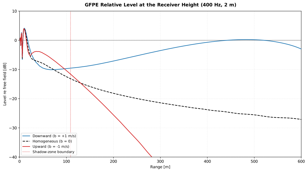
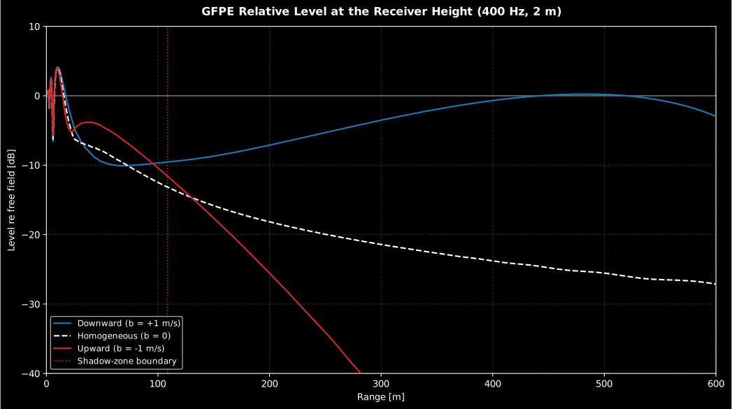
Whether refraction matters is mostly a question of range. A representative surface-layer gradient of ±0.1 s⁻¹ curves rays with a radius $R_c=c_0/|g|\approx 3.4$ km, so over the first hundred metres the paths are sensibly straight and the homogeneous models above are accurate. Beyond a few hundred metres the geometry takes over: downwind, or under a nocturnal temperature inversion, the downward-curved rays close over the ground and hold the level near (or even above) the homogeneous prediction, while upwind the same wind profile opens an acoustic shadow into which the level collapses by 20 dB or more (Attenborough & Van Renterghem 2021, Ch. 11). That is the familiar upwind/downwind asymmetry of any steady outdoor source: the same machine at the same distance, tens of decibels apart depending on which side you stand. It is also why ISO 9613-2 fixes its “favourable” downwind atmosphere by decree, and what its scalar $C_{met}$ compresses; the models on this page compute the physics that decides both.

1. Effective sound-speed profile

A moving (windy) atmosphere is well approximated by a non-moving one with the effective sound speed c_eff(z) = c(z) + u(z), the adiabatic sound speed plus the component of the wind in the propagation direction (Salomons Eq. 4.4). Two profile shapes cover most surface-layer cases:

• a linear profile c_eff(z) = c0 + g·z (linear_sound_speed_profile), the simplest refracting atmosphere and the one with exact ray geometry;
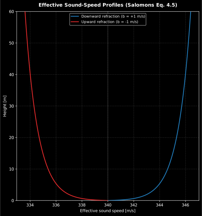
• the realistic logarithmic surface-layer profile c_eff(z) = c0 + b·ln(1 + z/z0) (log_linear_sound_speed_profile, Salomons Eq. 4.5), with b ≈ +1 m/s for a typical downward-refracting atmosphere, b ≈ -1 m/s for an upward-refracting one, and z0 the roughness length (about 0.1 m for grassland).

A positive gradient (sound speed increasing upward) bends rays down toward the receiver (favourable propagation); a negative gradient bends them up and opens an acoustic shadow near the ground.

from phonometry import log_linear_sound_speed_profile

profile = log_linear_sound_speed_profile(-1.0, ground_speed=340.0)  # upward
profile.speed_at(10.0)   # effective sound speed 10 m above the ground
profile.plot()           # c_eff(z) with height on the vertical axis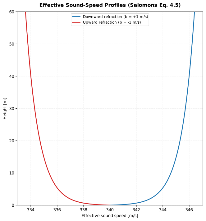

Show the code for this figure

import matplotlib.pyplot as plt
from phonometry import log_linear_sound_speed_profile

# The two canonical surface layers of Salomons Eq. 4.5 over grassland.
down = log_linear_sound_speed_profile(+1.0, ground_speed=340.0, max_height=60.0)
up = log_linear_sound_speed_profile(-1.0, ground_speed=340.0, max_height=60.0)
ax = down.plot(color="#1f77b4")
up.plot(ax=ax, color="#d62728")
plt.show()

2. Ray model

In geometrical acoustics a sound ray obeys Snell’s law cos(γ(z))/c(z) = const (Salomons Eq. 4.3). atmospheric_ray_paths integrates it with a fourth-order Runge-Kutta scheme, marching in range and reflecting specularly at the ground, and returns the curved paths, the turning points, the travel times and the number of ground reflections.

import numpy as np
from phonometry import atmospheric_ray_paths, log_linear_sound_speed_profile

profile = log_linear_sound_speed_profile(-1.0, ground_speed=340.0)
rays = atmospheric_ray_paths(profile, source_height=2.0,
                             launch_angles_deg=np.linspace(-8.0, 8.0, 17),
                             max_range=600.0)
rays.turning_points      # turning points per ray
rays.plot()              # the curved ray fan (needs matplotlib)

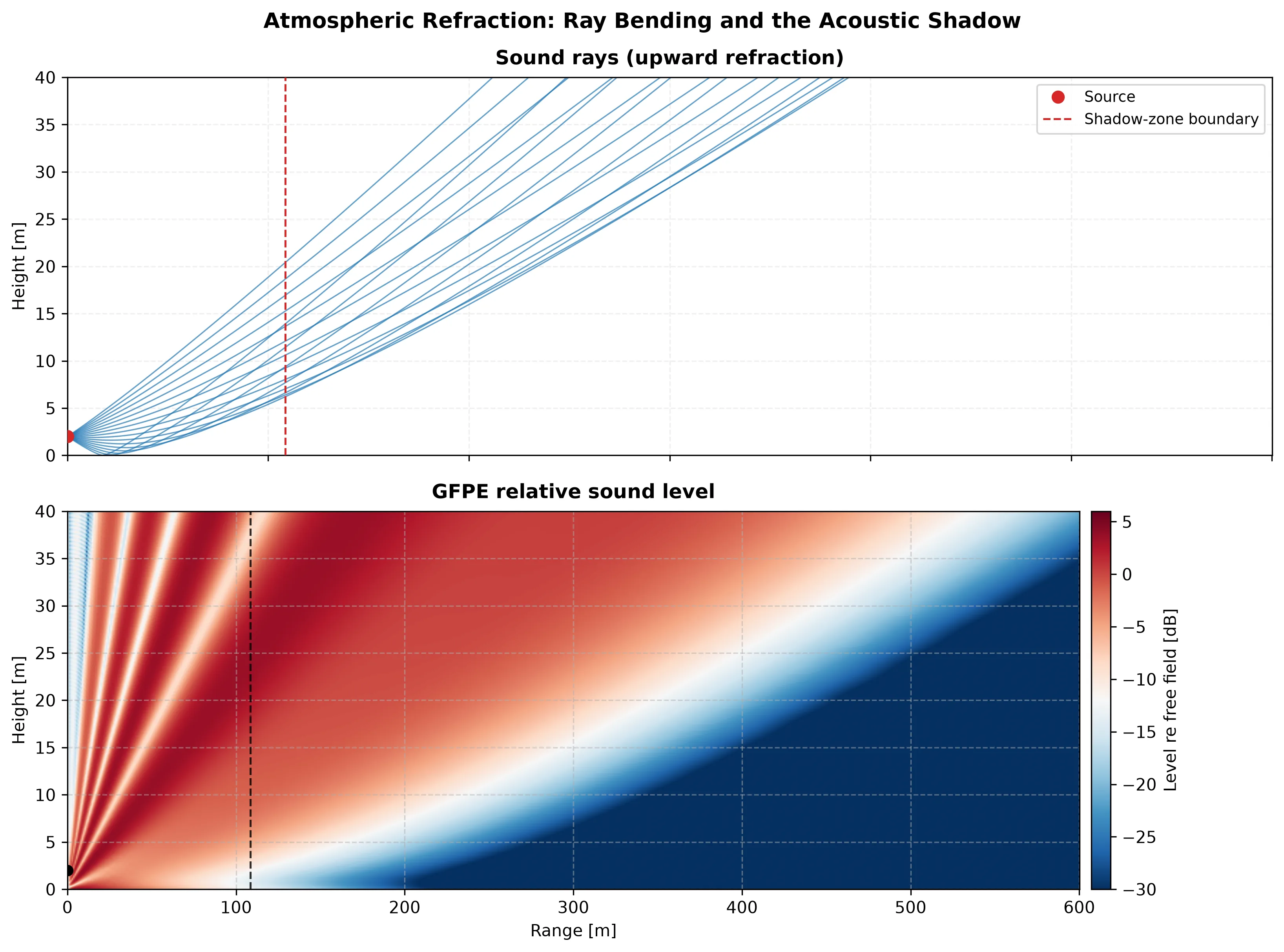
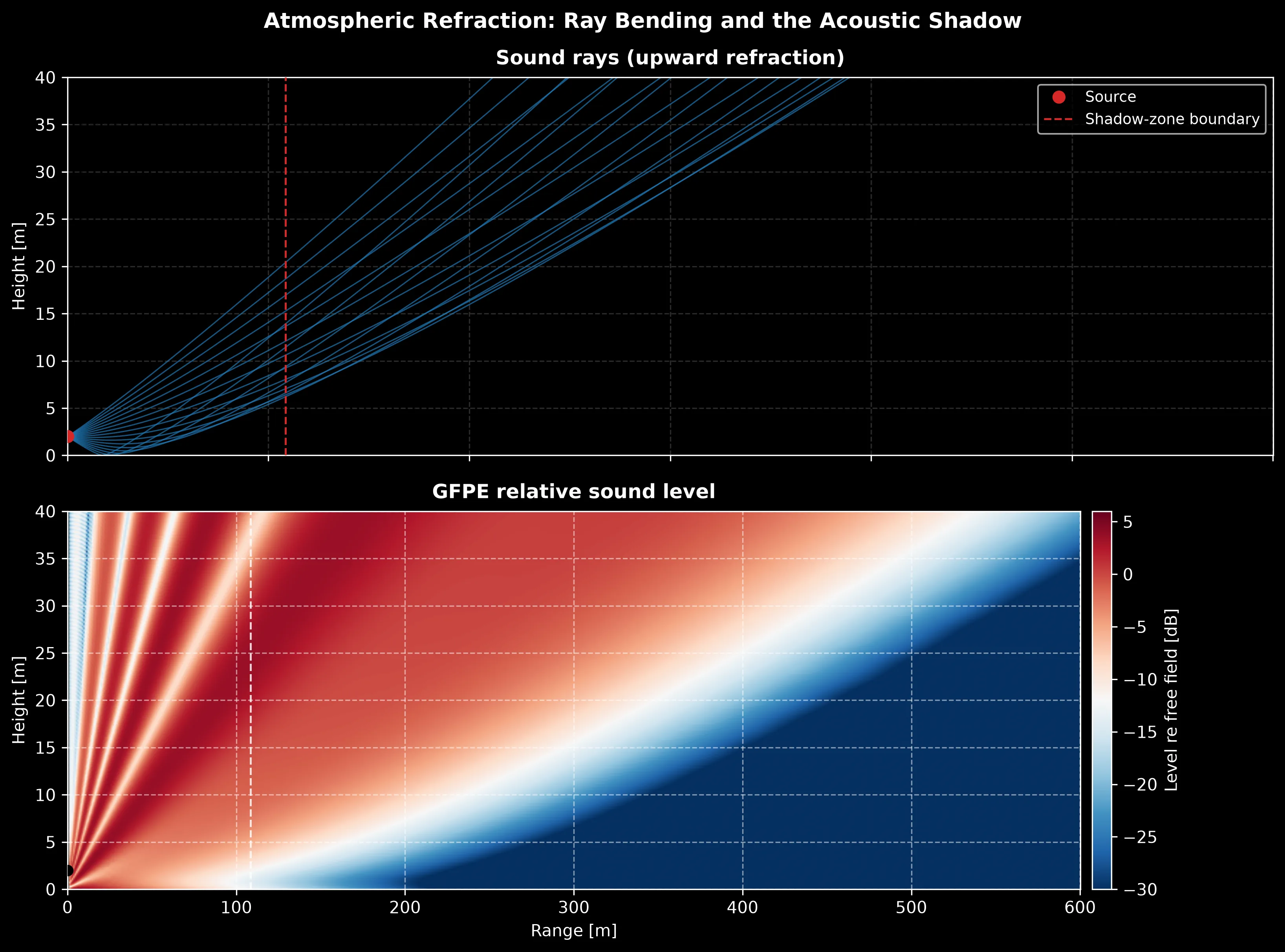
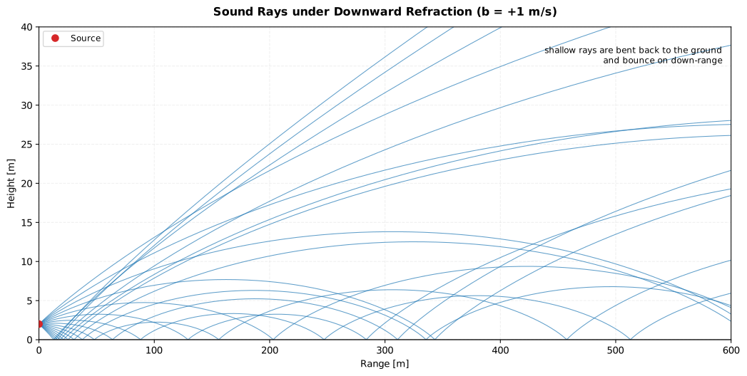
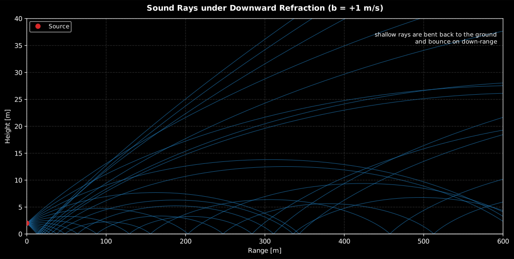
The page-top figure shows this upward-refracting fan opening its shadow. The favourable case is its mirror image: under downward refraction (b = +1) the shallow rays are bent back to the ground, bounce, and carry energy along the surface instead of losing it upward.

Show the code for this figure

import matplotlib.pyplot as plt
import numpy as np
from phonometry import atmospheric_ray_paths, log_linear_sound_speed_profile

# Downward refraction: the favourable-propagation mirror of the shadow case.
profile = log_linear_sound_speed_profile(+1.0, ground_speed=340.0)
rays = atmospheric_ray_paths(profile, source_height=2.0,
                             launch_angles_deg=np.linspace(-8.0, 8.0, 17),
                             max_range=600.0, n_steps=600)
rays.plot()   # shallow rays return to the ground and bounce on down-range
plt.show()

Closed-form geometry (linear gradient)

For a linear profile every ray is an exact circular arc of radius of curvature (Salomons Sec. 4.4; Attenborough Ch. 11):

$$R_c=\frac{c_0}{|g|\cos {\theta }_0},$$

exposed as ray_curvature_radius. A ray launched at angle θ0 in downward refraction turns at the height Rc(1 - cos θ0). For an upward-refracting linear profile the ground-grazing ray bounds a region beyond which no direct or once-reflected ray arrives, at the closed-form shadow-zone distance (shadow_zone_distance):

$$x_{\text{shadow}}=\sqrt{2R_c}\left(\sqrt{h_s}+\sqrt{h_r}\right),R_c=\frac{c_0}{|g|}.$$

These closed forms are the exact oracle for the ray tracer: a circle fit of a traced ray recovers Rc to machine precision.

3. Parabolic equation (Green’s Function PE)

The parabolic equation is the reference method for refraction and shadow zones at long range. It replaces the wave equation with a one-way (outgoing) equation valid within a limiting elevation angle, and marches it in range on a range-height grid. atmospheric_parabolic_equation implements the Green’s Function PE (GFPE, Salomons Appendix H), the atmospheric member of the same split-step Fourier family as the ocean parabolic_equation. Each range step transforms the field to the vertical-wavenumber domain, applies the free-space propagator together with the finite-impedance ground reflection R(kz) = (kz Z − k0)/(kz Z + k0) (Salomons Eq. H.28), transforms back, adds the surface-wave residue of the reflection pole (the third term of Eq. H.49) and applies the refraction phase screen exp(i Δr (k(z) − ka)) (Eq. H.58). The source is a Gaussian starter with its ground image (Eqs. G.64, G.76) and an absorbing layer at the top of the grid suppresses top-boundary reflections. The result is the relative sound level ΔL(z, r) = 20 lg(|p| R1) (dB re free field) over the whole range-height plane.

from phonometry import atmospheric_parabolic_equation, log_linear_sound_speed_profile

profile = log_linear_sound_speed_profile(-1.0, ground_speed=340.0)  # upward
pe = atmospheric_parabolic_equation(400.0, profile, source_height=2.0,
                                    flow_resistivity=200e3,  # grassland
                                    max_range=600.0, max_height=40.0)
pe.level_at_height(2.0)   # relative level vs range at 2 m
pe.plot()                 # the range-height relative-level field (needs matplotlib)

Cut the field at the receiver height and the whole story of this page is one figure: with everything else identical, the sign of the gradient alone moves the 400 Hz level at 600 m by more than 30 dB.

Show the code for this figure

import warnings

import matplotlib.pyplot as plt

from phonometry import (
    atmospheric_parabolic_equation,
    linear_sound_speed_profile,
    log_linear_sound_speed_profile,
    shadow_zone_distance,
)

cases = [
    (log_linear_sound_speed_profile(+1.0, ground_speed=340.0), "Downward (b = +1 m/s)"),
    (linear_sound_speed_profile(0.0, ground_speed=340.0), "Homogeneous (b = 0)"),
    (log_linear_sound_speed_profile(-1.0, ground_speed=340.0), "Upward (b = -1 m/s)"),
]
fig, ax = plt.subplots(figsize=(11, 6.2))
with warnings.catch_warnings():
    warnings.simplefilter("ignore")
    for profile, label in cases:
        pe = atmospheric_parabolic_equation(400.0, profile, source_height=2.0,
                                            flow_resistivity=200e3,
                                            max_range=600.0, max_height=40.0)
        ax.plot(pe.ranges, pe.level_at_height(2.0), label=label)
# The closed-form boundary of the equivalent linear upward gradient (its
# 10 m mean), the dotted line of the figure.
up = cases[2][0]
grad = float(up.speed_at(10.0) - 340.0) / 10.0
ax.axvline(shadow_zone_distance(grad, 2.0, 2.0, ground_speed=340.0),
           color="k", ls=":", label="Shadow-zone boundary")
ax.set(xlabel="Range [m]", ylabel="Level re free field [dB]", ylim=(-40, 10))
ax.legend()
plt.show()

The ground impedance is supplied directly (impedance=, a normalized complex value in the e^{-iωt} convention of Salomons, with Im(Z) > 0 for a passive ground), as a PorousMediumResult, or from an effective flow_resistivity via the porous models of the materials domain; the porous models work in the opposite e^{+jωt} convention, so their impedance is conjugated internally.

Show the code for this figure

import warnings

import matplotlib.pyplot as plt
import numpy as np

from phonometry import (
    atmospheric_parabolic_equation,
    atmospheric_ray_paths,
    log_linear_sound_speed_profile,
    shadow_zone_distance,
)

c0 = 340.0
profile = log_linear_sound_speed_profile(-1.0, ground_speed=c0, max_height=60.0)
zs = 2.0
fig, axes = plt.subplots(2, 1, figsize=(11, 8.2), sharex=True)

rays = atmospheric_ray_paths(profile, source_height=zs,
                             launch_angles_deg=np.linspace(-8.0, 8.0, 17),
                             max_range=600.0, n_steps=3000)
for i in range(rays.heights.shape[0]):
    axes[0].plot(rays.ranges[i], rays.heights[i], color="#1f77b4", lw=0.8, alpha=0.7)
axes[0].plot([0.0], [zs], "o", color="#d62728", label="Source")
grad = (profile.speed_at(10.0) - c0) / 10.0
x_sh = shadow_zone_distance(float(grad), zs, zs, ground_speed=c0)
axes[0].axvline(x_sh, color="#d62728", ls="--", label="Shadow-zone boundary")
axes[0].set(ylabel="Height [m]", ylim=(0, 40), title="Sound rays (upward refraction)")
axes[0].legend()

with warnings.catch_warnings():
    warnings.simplefilter("ignore")
    pe = atmospheric_parabolic_equation(400.0, profile, source_height=zs,
                                        flow_resistivity=200e3,
                                        max_range=600.0, max_height=40.0)
img = axes[1].imshow(pe.relative_level, cmap="RdBu_r", vmin=-30, vmax=6,
                     aspect="auto", origin="lower", interpolation="bilinear",
                     extent=(pe.ranges[0], pe.ranges[-1], pe.heights[0], pe.heights[-1]))
axes[1].axvline(x_sh, color="k", ls="--")
axes[1].set(ylabel="Height [m]", xlabel="Range [m]", ylim=(0, 40),
            title="GFPE relative sound level")
fig.colorbar(img, ax=axes[1], label="Level re free field [dB]")
plt.tight_layout()
plt.show()

4. Validation

The models are anchored by independent oracles, pinned numerically in the conformance report (section “Atmospheric refraction”):

• Homogeneous limit → spherical ground effect. With a zero gradient the GFPE field reproduces the exact Weyl-Van der Pol ground_effect at every range, to a few tenths of a dB over grassland on the default grid, and to the coherent +6 dB two-ray enhancement over a rigid ground.
• Exact ray geometry. For a linear profile the traced ray is a circular arc whose fitted radius matches ray_curvature_radius to machine precision.
• Reciprocity. Swapping the source and receiver heights leaves the PE level.
• Shadow zone. Over an upward-refracting profile the PE level collapses far inside the closed-form shadow distance.

What this guide covers

Covered. The ray model (Runge-Kutta integration of Snell’s law, atmospheric_ray_paths) with the closed-form linear-profile geometry (ray_curvature_radius, shadow_zone_distance, Salomons Sec. 4.4), and the Green’s Function parabolic equation (atmospheric_parabolic_equation, Salomons Appendices G and H): the Gaussian starter, the finite-impedance ground reflection, the refraction phase screen and the absorbing top layer. Validated by the homogeneous limit against the exact spherical ground effect (a few tenths of a dB, and the +6 dB rigid-ground enhancement), exact ray geometry to machine precision, reciprocity and the shadow-zone collapse.

Not covered. Both models take a single effective-sound-speed profile that varies with height alone, not with range: a horizontally inhomogeneous atmosphere (a gradient that changes along the path) sits outside their range-independent formulation, described in the module as the counterpart of the “range-independent ocean solvers” it mirrors. Both also assume flat ground at z = 0; neither takes a terrain elevation profile.

References

• Attenborough, K., & Van Renterghem, T. (2021). Predicting outdoor sound (2nd ed.). CRC Press. https://doi.org/10.1201/9780429470141Chapter 11 (refraction by wind and temperature gradients, ray models and shadow zones). ISBN 978-1-138-30655-2.
• Salomons, E. M. (2001). Computational atmospheric acoustics. Kluwer Academic. https://doi.org/10.1007/978-94-010-0660-6Chapter 4 (effective sound speed, the ray model and PE examples), Appendix G (the Crank-Nicholson PE and the Gaussian starter, Eqs. G.64, G.76) and Appendix H (the Green's Function PE, the impedance reflection Eq. H.28 and the refraction factor Eq. H.58). ISBN 978-1-4020-0390-5.