Swept-sine distortion and phase utilities

A single exponential sine sweep characterises the linear response and every harmonic distortion order of a weakly nonlinear system at once. After deconvolution, the distortion products of order n pack into separate impulse responses that precede the linear response by the fixed advance (Farina 2000)

$$\Delta t_n=T\frac{\ln n}{\ln (f_2/f_1)}=L\ln n,L=\frac{T}{\ln (f_2/f_1)},$$

so windowing each arrival yields the higher harmonic frequency responses H1(f), H2(f), ..., HN(f) and, from them, the total harmonic distortion as a function of the excitation frequency with one sweep instead of a tone-by-tone stepping. This page covers that separation in phonometry.electroacoustics, with the phase-coherent synchronized sweep of Novak, Lotton & Simon (2015) as the default, and the companion phase utilities in phonometry.metrology: minimum phase from |H|, group delay and excess phase.

1. One sweep, every harmonic

For an exponential sweep the instantaneous frequency rises as f(t) = f1·e^(t/L), so the moment the excitation passes f, the n-th harmonic distortion product appears at n·f: exactly where the sweep itself will be L·ln(n) seconds later. Deconvolving the recording against the sweep therefore time-compresses each order into its own impulse response, L·ln(n) before the linear one. swept_sine_distortion windows each arrival (with the exact fractional-sample alignment), Fourier transforms it into Hn(f), and reads the distortion of order n at excitation frequency f from |Hn(n·f)|:

$$\mathrm{THD}(f)=\frac{\sqrt{{\sum }_{n\ge 2}|H_n(nf){|}^2}}{|H_1(f)|}.$$

import numpy as np
from phonometry import swept_sine_distortion, synchronized_sweep_signal

fs, f1, f2, seconds = 48000, 20.0, 6000.0, 4.0
x = synchronized_sweep_signal(fs, f1, f2, seconds)   # play this...
# ... record the device response into `y` (include the decay tail) ...
res = swept_sine_distortion(y, fs, f1, f2, seconds, n_harmonics=3)

res.harmonic_responses    # complex H1..H3 on res.frequencies
res.thd, res.thd_frequencies
res.distortion_ratios     # |Hn(n f)| / |H1(f)| per order
res.plot()                # |Hn| magnitudes + THD(f)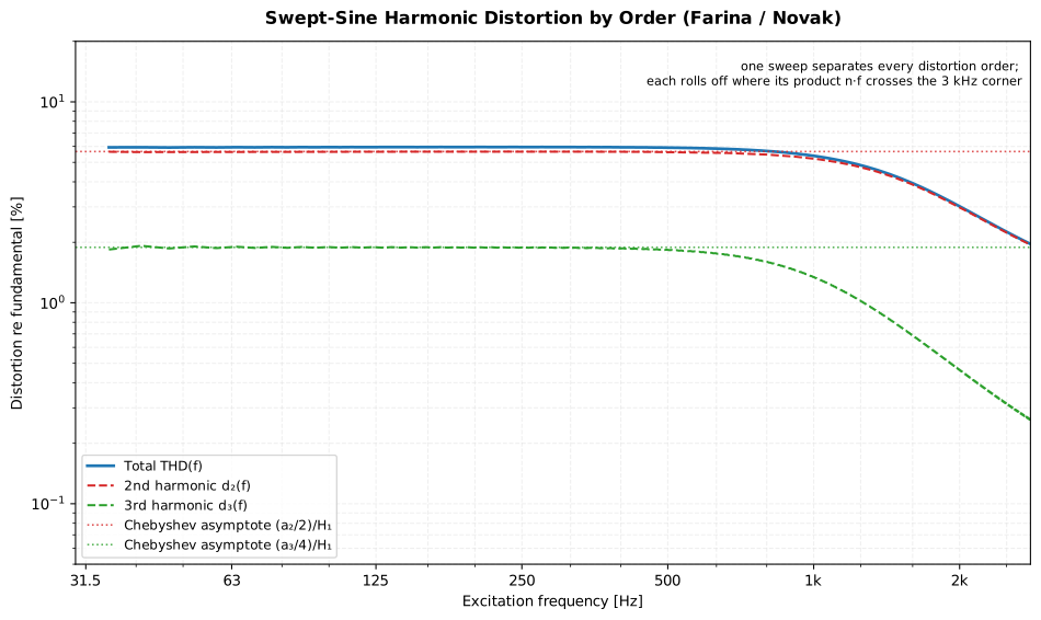

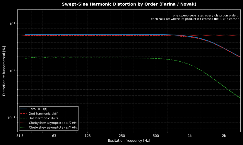
Show the code for this figure

import matplotlib.pyplot as plt
import numpy as np
from scipy import signal as sp_signal
from phonometry import swept_sine_distortion, synchronized_sweep_signal

fs, f1, f2, seconds = 48000, 20.0, 6000.0, 4.0
a2, a3 = 0.12, 0.08
x = synchronized_sweep_signal(fs, f1, f2, seconds)
b, a = sp_signal.butter(2, 3000.0, fs=fs)             # 3 kHz post-filter
y = sp_signal.lfilter(b, a, x + a2 * x**2 + a3 * x**3)
res = swept_sine_distortion(y, fs, f1, f2, seconds, n_harmonics=3)

h1 = 1.0 + 3.0 * a3 / 4.0                              # Chebyshev gain
fig, ax = plt.subplots(figsize=(10, 6))
ax.loglog(res.thd_frequencies, 100.0 * res.thd, label="Total THD(f)")
ax.loglog(res.thd_frequencies, 100.0 * res.distortion_ratios[0],
          ls="--", label="2nd harmonic d2(f)")
ax.loglog(res.thd_frequencies, 100.0 * res.distortion_ratios[1],
          ls="--", label="3rd harmonic d3(f)")
ax.axhline(100.0 * (a2 / 2.0) / h1, ls=":",
           label="Chebyshev asymptote (a2/2)/H1")
ax.axhline(100.0 * (a3 / 4.0) / h1, ls=":",
           label="Chebyshev asymptote (a3/4)/H1")
ax.set_xlabel("Excitation frequency [Hz]")
ax.set_ylabel("Distortion re fundamental [%]")
ax.legend()
plt.show()

The oracle behind the implementation is the memoryless polynomial: driving y = x + a2·x² + a3·x³ with a unit sweep must return, by the Chebyshev identities, |H1| = 1 + 3a3/4, |H2| = a2/2 (phase -π/2), |H3| = a3/4 (phase π) and THD = √((a2/2)² + (a3/4)²)/(1 + 3a3/4). The test and conformance suites pin all four, and the same THD measured tone by tone with phonometry.thd agrees to 0.1 %.

2. The synchronized sweep (Novak et al. 2015)

Windowing separates the harmonic magnitudes with any exponential sweep, but the phases of H2..HN are only meaningful if delaying the sweep by L·ln(n) is exactly equivalent to generating its n-th harmonic. That holds only for

$$x(t)=\sin \left[2\pi f_{1}L{e}^{t/L}\right],L=\frac{1}{f_1}\mathrm{round}\left(\frac{f_1\tilde{T}}{\ln (f_2/f_1)}\right),$$

the synchronized swept-sine: the rounding makes f1·L an integer, so the sweep starts at zero phase and every harmonic copy lines up. synchronized_sweep_signal generates it (the duration is quantized slightly; when f2/f1 is an integer the sweep also ends at zero phase), and swept_sine_distortion(..., method="synchronized"), the default, deconvolves with the closed-form spectrum of the inverse filter,

$$\tilde{X}(f)=2\sqrt{f/L}{e}^{-j2\pi fL(1-\ln (f/f_1))+j\pi /4},$$

rather than an FFT of the signal. Besides being exact, the analytic deconvolution extends the usable band of each Hn to [n·f1, n·f2] (Novak et al., Fig. 6): the second harmonic of a 6 kHz sweep is measured up to 12 kHz.

Two practical notes from the paper are built in: the recording mean is subtracted by default (remove_dc=True; a DC offset otherwise leaks a scaled inverse filter into the impulse response), and the non-integer part of each arrival L·ln(n)·fs is removed in the frequency domain, so the harmonic phases carry no residual sub-sample skew.

3. Analysing classical ESS recordings (method="farina")

Recordings made with the plain exponential sweep of phonometry.sweep_signal (the ISO 18233 excitation used by impulse_response) are analysed with method="farina": the same windowing over the time-reversed, amplitude-compensated inverse filter of Farina (2000). The harmonic magnitudes and the THD are correct (the Chebyshev oracle passes identically), but the sweep’s -1 phase term breaks the time-shift equivalence, so the phases of H2..HN depend on the excitation and should be ignored; the band of every Hn is also capped at f2 by the inverse filter.

from phonometry import sweep_signal, swept_sine_distortion

x = sweep_signal(fs, f1, f2, seconds)          # the ISO 18233 ESS
res = swept_sine_distortion(y, fs, f1, f2, seconds, method="farina")
res.plot()   # same |Hn| + THD(f) panels as the synchronized method (needs matplotlib)

The result is the same plottable SweptSineDistortionResult as the synchronized method, so the |Hn| and THD(f) panels of the section-1 figure read identically; only the harmonic phases (and the top of each order’s band) differ between the two methods.

Sizing rules for both methods: the closest pair of arrivals is spaced L·ln(N/(N-1)) seconds, so the per-order window (ir_length, default the largest power of two that fits, capped at 8192 samples) must not exceed it: lengthen the sweep or lower n_harmonics for reverberant systems whose tails need longer windows. Keep n_harmonics·f2 below Nyquist: distortion products above it fold back in any real recording. The analysis is referenced to the excitation amplitude, so H1 is the linear gain and the THD is level-referenced exactly as driven.

4. Phase utilities: minimum phase, group delay, excess phase

For a causal, stable, minimum-phase system the log-magnitude and phase of the frequency response are a Hilbert-transform pair (Bendat & Piersol, Sec. 13.1.4): the phase is fully determined by |H(f)|. The phonometry.metrology utilities compute that reconstruction with the real cepstrum and decompose any measured response into its invertible and all-pass parts:

import numpy as np
from phonometry import (
    excess_phase, group_delay, minimum_phase, phase_decomposition,
)

H = np.fft.rfft(ir)                    # one-sided response, DC..Nyquist
h_min = minimum_phase(np.abs(H))       # phase from the magnitude alone
tau_g = group_delay(H, fs)             # -(1/2pi) dphi/df, seconds
phi_x = excess_phase(H)                # unwrap(arg H) - phi_min

res = phase_decomposition(H, fs)       # everything on one axis
res.excess_group_delay                 # the all-pass part, in seconds
res.plot()                             # magnitude, phases, group delays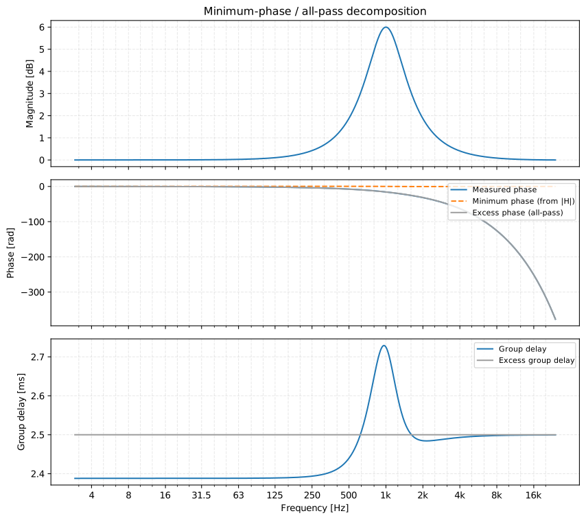

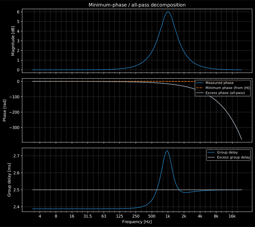
A +6 dB peaking equalizer measured through a 2.5 ms processing latency: the minimum-phase part carries only the small phase wiggle an equalizer could invert, the excess phase is the pure −2πf·t₀ ramp of the delay, and the excess group delay reads the latency directly as a flat 2.5 ms line.

Show the code for this figure

import matplotlib.pyplot as plt
import numpy as np
from scipy import signal as sp_signal
from phonometry import phase_decomposition

fs = 48000.0
delay = int(0.0025 * fs)                      # a 2.5 ms processing latency
gain_a = 10.0 ** (6.0 / 40.0)                 # +6 dB peaking EQ at 1 kHz, Q = 1
w0 = 2.0 * np.pi * 1000.0 / fs
alpha = np.sin(w0) / 2.0
b = np.array([1 + alpha * gain_a, -2 * np.cos(w0), 1 - alpha * gain_a])
a = np.array([1 + alpha / gain_a, -2 * np.cos(w0), 1 - alpha / gain_a])
imp = np.zeros(16384)
imp[delay] = 1.0
ir = sp_signal.lfilter(b / a[0], a / a[0], imp)

res = phase_decomposition(np.fft.rfft(ir), fs)
res.plot()   # |H|, the three phases and the group delays
plt.show()

The decomposition H = H_min · H_ap splits what an equalizer can invert (H_min, minimum phase, causal and causally invertible) from what it never can (H_ap, the all-pass excess: latency plus non-minimum-phase zeros such as reflections). The excess phase is 0 for a minimum-phase response and exactly -2πf·t0 for a pure latency t0; its group delay reads the latency in seconds.

Numerical contract, pinned by the tests: on a strictly minimum-phase biquad sampled on a dense grid the reconstructed phase matches the true phase to better than 1e-12 rad; the group delay of a first-order allpass matches the closed form (1-a²)/(1+2a·cosω+a²) to 1e-5 samples; the excess group delay of a delayed biquad returns the delay to 1e-6 samples. The precautions are documented with the API: the response must be sampled uniformly from DC to Nyquist inclusive (the rfft layout) and densely enough that the underlying impulse response fits the implied record; magnitude zeros (band-pass edges, notch bottoms) are floored and are not representable by a minimum-phase system; the oversample factor (trigonometric interpolation of the magnitude before the cepstrum) mitigates the cepstral aliasing that near-circle zeros cause on coarse grids.

Relation to other tools

• impulse_response recovers the linear IR from the same sweep recording and simply discards the negative-time distortion products; swept_sine_distortion is the tool that reads them.
• thd / harmonic_analysis measure distortion from a steady tone at one frequency; the sweep separator returns the same ratios as a continuous function of frequency, from one measurement.
• The phase utilities operate on any one-sided complex response: an rfft of a measured IR, or the response of a transfer_function estimate on a uniform grid. minimum_phase alone also accepts a plain magnitude array, e.g. a design target for equalization.

What this guide covers

Covered. Farina’s exponential-sweep deconvolution (AES preprint 5093, 2000) and the phase-coherent synchronized swept-sine of Novak, Lotton & Simon (2015): the harmonic separation, the closed-form inverse-filter spectrum and the fractional-sample de-skewing, implemented by swept_sine_distortion and synchronized_sweep_signal. The phase utilities minimum_phase, group_delay, excess_phase and phase_decomposition implement the Hilbert-transform relation of Bendat & Piersol Section 13.1.4 through the real cepstrum.

Not covered. Intermodulation and dynamic intermodulation distortion (IEC 60268-3, clauses 14.12.7-10) are measured from steady tones on the electroacoustics page, not from a sweep; this page separates harmonic orders only. Müller & Massarani’s sweep monograph is cited for background practice (fades, inverse-filter technique), not for a specific implemented formula. With method="farina", the harmonic phases of H2..HN are returned but should be ignored: the plain exponential sweep breaks the time-shift/harmonic equivalence the synchronized method relies on.

References

• Bendat, J. S., & Piersol, A. G. (2010). Random data: Analysis and measurement procedures (4th ed.). Wiley. https://doi.org/10.1002/9781118032428Section 13.1.4: the Hilbert-transform relation between log-magnitude and phase behind the minimum-phase reconstruction. ISBN 978-0-470-24877-5.
• Farina, A. (2000). Simultaneous measurement of impulse response and distortion with a swept-sine technique (108th AES Convention, Paris, preprint 5093). The exponential-sweep deconvolution and the L·ln(n) packing of each distortion order ahead of the linear impulse response.
• Müller, S., & Massarani, P. (2001). Transfer-function measurement with sweeps. Journal of the Audio Engineering Society, 49(6), 443-471. The sweep-measurement monograph behind the practice notes: inverse filters, fades and the rejection of distortion from the linear impulse response.
• Novak, A., Lotton, P., & Simon, L. (2015). Synchronized swept-sine: Theory, application and implementation. Journal of the Audio Engineering Society, 63(10), 786-798. https://doi.org/10.17743/jaes.2015.0071The synchronization condition that makes harmonic phases system properties, the closed-form inverse-filter spectrum used for the deconvolution and the fractional-sample separation.