Speech Transmission Index (STI)

A public-address system, an intercom, a reverberant lecture hall: each is a transmission channel between a talker’s mouth and a listener’s ear, and each degrades speech in its own way. The Speech Transmission Index (STI) of IEC 60268-16 rates that channel with a single number in [0, 1] by measuring how much of the speech envelope survives the trip. This page covers the modulation-transfer physics behind the index, the indirect method from a measured room impulse response, and the direct STIPA measurement with its standardized test signal.

Note

STI vs SII. The STI characterises a transmission channel (how much of the speech modulation a room or sound system preserves) while the SII predicts intelligibility from audibility: how much of the speech spectrum clears the noise and the hearing threshold at the listener’s ear. For the latter, see the Speech Intelligibility Index guide.

How do I compute the IEC 60268-16 Speech Transmission Index in Python?

From a measured room impulse response, call hearing.sti_from_impulse_response(ir, fs, snr=25.0). The result gives sti on the 0 to 1 scale, its Annex F rating letter and the seven octave-band modulation transfer indices. For a direct measurement, play hearing.stipa_signal(fs) in the room and pass the recording to hearing.stipa(recording, fs).

1. The modulation transfer function

Reverberation and noise do not muffle speech uniformly; they blur its envelope: the slow (0.63–12.5 Hz) intensity modulations that carry syllables. STI quantifies how much of that modulation survives from mouth to ear, per octave band, as the modulation transfer function m(F). A delta-like channel keeps m = 1 (STI = 1); reverberation low-passes the envelope following Schroeder’s closed form, and steady noise scales it:

$$m(F)=\frac{1}{\sqrt{1+{\left(2\pi F\frac{T_{60}}{13.8}\right)}^2}}\cdot \frac{1}{1+10^{-\mathrm{SNR}/10}}$$

Modulation depth is the thing worth measuring because intelligibility rides on the depth of the envelope valleys, not on the loudness of the peaks. A talker alternates energy bursts (vowels) with near-silences (stop gaps, fricative onsets) at syllable rate, and a listener segments speech by hearing those dips. A reverberant tail fills the dips from behind, since late energy smears into the gaps; steady noise raises their floor. In both cases the received modulation depth shrinks, and with it the contrast between speech sounds, even when the average level barely changes. The full method probes m(F) at 14 modulation frequencies (0.63 Hz to 12.5 Hz in one-third-octave steps) in each of the 7 octave bands from 125 Hz to 8 kHz, converts each m to an effective signal-to-noise ratio clipped to ±15 dB, and combines the results, band-weighted, into the index: the STI is an effective SNR of the envelope, mapped onto [0, 1].

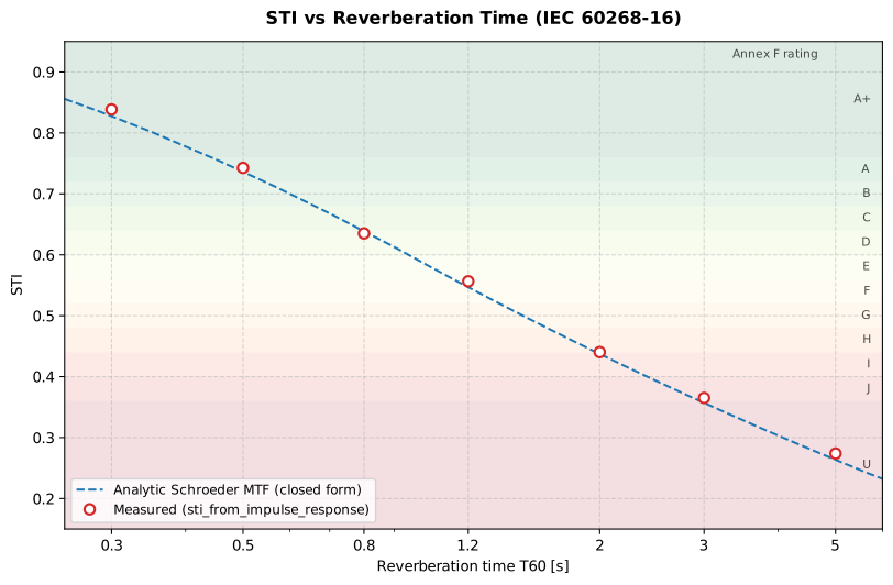
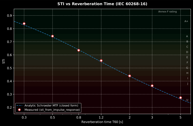
Show the code for this figure

import numpy as np
import matplotlib.pyplot as plt
from phonometry import hearing

fs = 48000

# STI vs reverberation time: sweep hearing.sti_from_impulse_response over synthetic
# exponential decays (white noise x exp(-6.9077 t / T60)) at a T60 grid,
# exactly the physics behind the curve above:
rng = np.random.default_rng(0)
t60_grid = np.array([0.3, 0.5, 0.8, 1.2, 1.6, 2.0, 2.5, 3.0, 4.0, 5.0])
sti_values = []
for t60 in t60_grid:
    t = np.arange(int(2 * t60 * fs)) / fs
    ir = rng.standard_normal(t.size) * np.exp(-6.9077 * t / t60)
    sti_values.append(hearing.sti_from_impulse_response(ir, fs).sti)

fig, ax = plt.subplots()
ax.semilogx(t60_grid, sti_values, "o-")
ax.set_xlabel("Reverberation time T60 [s]")
ax.set_ylabel("STI")
ax.set_ylim(0.0, 1.0)
ax.grid(True, which="both", alpha=0.3)
plt.show()

2. Indirect and direct (STIPA) measurement

import numpy as np
from phonometry import hearing

fs = 48000
# A measured room impulse response (synthesized decay so the example runs)
ir = np.random.default_rng(0).standard_normal(fs) * np.exp(-6.9 * np.arange(fs) / fs / 0.5)

# Indirect method: from a measured room impulse response
res = hearing.sti_from_impulse_response(ir, fs, snr=25.0)
print(f"STI = {res.sti:.2f}  ({res.rating})")   # e.g. 0.62 (D)

# Direct STIPA measurement: play hearing.stipa_signal() in the room, record it
test = hearing.stipa_signal(fs, seconds=18.0, level_db=80.0)
recording = test                       # in practice, the microphone signal after playback
res = hearing.stipa(recording, fs)
res.plot()   # per-band modulation transfer index (MTI) bars, STI + rating in the title

Whichever route produced it, the result is worth reading band by band before the single number is quoted: the STI is a weighted combination of seven octave-band modulation transfer indices, and a room usually fails in a particular part of the spectrum rather than uniformly.

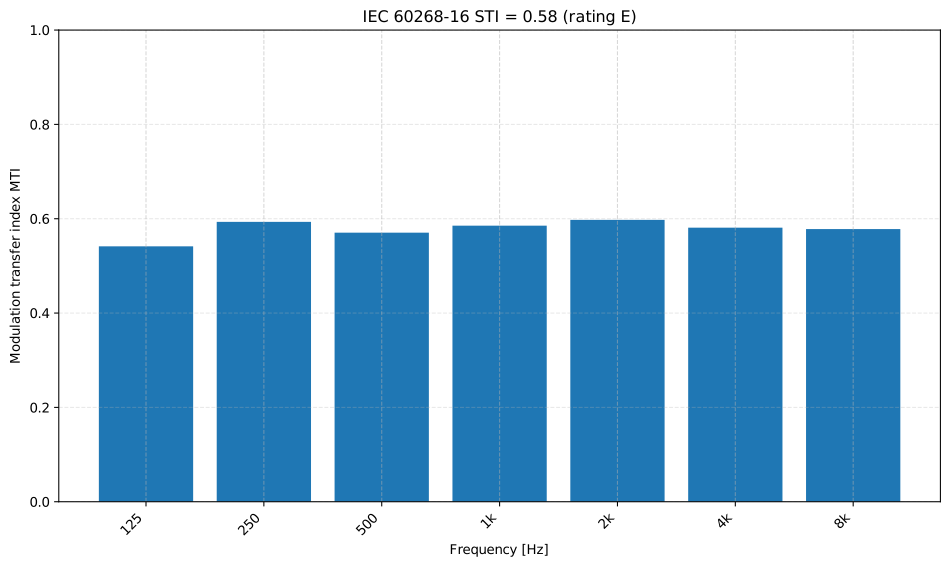
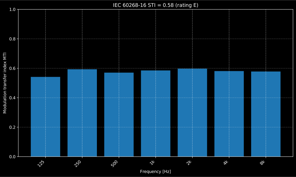
Show the code for this figure

import numpy as np
import matplotlib.pyplot as plt
from phonometry import hearing

# A reverberant hall (T60 = 0.9 s) measured with a 15 dB speech-to-noise
# ratio: a synthesized exponential decay stands in for the measured IR.
fs = 48000
rng = np.random.default_rng(0)
n = np.arange(fs)
ir = rng.standard_normal(fs) * np.exp(-6.9078 * n / fs / 0.9)
res = hearing.sti_from_impulse_response(ir, fs, snr=15.0)
print(round(res.sti, 3), res.rating)      # 0.583 E

# One line: the per-band MTI bars with the STI and its rating in the title.
res.plot()
plt.show()

# By hand, mirroring what STIResult.plot() draws:
bands = [125, 250, 500, 1000, 2000, 4000, 8000]
fig, ax = plt.subplots()
ax.bar(np.arange(len(bands)), res.mti)
ax.set_xticks(np.arange(len(bands)))
ax.set_xticklabels([f"{b}" for b in bands])
ax.set_xlabel("Frequency [Hz]")
ax.set_ylabel("Modulation transfer index MTI")
ax.set_ylim(0.0, 1.0)
ax.set_title(f"STI = {res.sti:.2f} (rating {res.rating})")
plt.show()

In this hall the seven indices sit within 0.06 of each other, the signature of a decay that is uniform across the spectrum plus a broadband noise floor. A profile that sags at 125 Hz and 250 Hz instead points at low-frequency reverberation (too little bass absorption), while one that falls only at 4 kHz and 8 kHz usually means the loudspeaker is out of the listener’s direct-sound coverage, since air and directivity strip the top bands first. Those are different remedies, and only the per-band view distinguishes them.

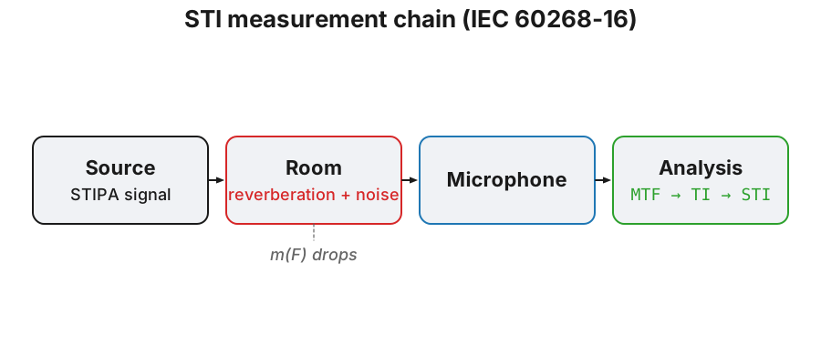
The direct measurement sends the STIPA signal along the full chain drawn below, from the source through the room to the microphone and into the per-band modulation analysis that yields the index.

stipa emits a UserWarning when the recording is shorter than the recommended 15 s (IEC 60268-16 STIPA practice, 15 s to 25 s): below that the slow modulation components are averaged over too few periods and the STI is biased low (an ideal loopback gives STI ≈ 0.956 at 5 s vs ≈ 0.998 at 18 s).

The implementation follows Edition 5 (2020): Edition 4’s normative PDF is the base and every Ed. 5 change is source-attributed in the code; the only numeric delta is the revised male speech spectrum of clause A.6.1. CI checks the standard’s own verification vectors: the six weighting-factor band pairs to ±0.001 STI, the m ↔ STI mapping table, the level-dependent masking control points, and Schroeder-form decays at four T₆₀ values.

The analyzer is also verified end to end against the IEC 60268-16 rev 5 verification test bench signals from stipa.info (Embedded Acoustics BV): the direct-method modulation-depth staircase (Annex C.3.2), the indirect-method exponential decays against the closed-form Schroeder MTF (C.3.3), the filter-bank slope test with a +41 dB unmodulated adjacent-octave tone (C.4.2, m ≥ 0.5), the weighting-factor band pairs (A.2.2) and the filter-bank phase-distortion test with half-octave edge carriers (A.3.1.2, |STI bias| < 0.01 over TI = 0.1–0.9). All five suites pass with the level-dependent features disabled, as the bench prescribes. The 49 certified WAVs stay local (third-party data, not committed); CI re-derives the same signal constructions synthetically in the conformance suite.

Direct or indirect: choosing between them

Each route has failure modes the standard is explicit about:

• Non-linear or time-variant channels. The indirect method assumes a linear, time-invariant channel: an impulse response cannot represent clipping, compressors, automatic gain control or a vocoder. For a sound system with non-linear processing in the chain, measure directly: the STIPA signal at least travels through the real chain, and the FULL STI signal is the reliable choice where the distortion is severe (IEC 60268-16 clause 6.3 and Table 3).
• Level-dependent effects. The STI is not level-invariant: auditory masking and the reception threshold act on the absolute band levels at the listener. Play the test signal at the system’s operating level (the standard’s Annex J practice sets it 3 dB above the L_Aeq of continuous speech at the position) and pass level= and ambient= so the analysis includes them; an impulse response measured loud and rescaled afterwards misses these effects entirely.
• Impulsive and fluctuating background noise. A dropped tool or babble during a direct measurement corrupts the measured modulation depths (clause 7.13). The standard’s remedy is the indirect route: average the impulse response with MLS or sweeps for a noise-free MTF, then add the noise degradation back via snr= or level=/ambient=. A quick sanity check is to run the analyzer with the source off; the residual STI should stay below 0.20.
• Statistical spread. The STIPA signal is pseudo-random noise, so repeated direct measurements scatter by up to about 0.03 STI even in steady conditions (and more in fluctuating noise); repeat and compare rather than trusting a single run, and respect the minimum duration flagged by the UserWarning above.

sti_from_impulse_response() / stipa() parameters

Parameter	Type	Units	Range / default	Notes
ir / x	1D array	any / Pa	non-empty	IR (indirect) or STIPA recording (direct)
fs	int	Hz	> 0
snr	float or 7-vector, optional	dB	default None	Adds steady-noise degradation
level	7-vector, optional	dB SPL	default None	Enables auditory masking + reception threshold (Tables A.2/A.3)
ambient	7-vector, optional	dB SPL	needs level	Ambient noise band levels
reference	1D array, optional (stipa)	—	default None	Measured source signal instead of the nominal m = 0.55

Both return STIResult: sti, mti (7 bands), mtf (7×14 or 7×2), band_levels, rating (Annex F letter A+…U).

IEC 60268-16 report (.report())

STIResult.report(path) renders a one-page PDF fiche laid out like a voice-alarm / public-address intelligibility verification report: a standard-basis line stating the measurement method (the full STI indirect method from an impulse response, or the direct STIPA method on a recorded signal), an optional metadata header block, a per-octave-band modulation transfer index table beside the per-band MTI bars (the result’s own .plot()), the boxed STI = X single number with the Annex F qualification band, an optional verdict row and a footer with the fixed disclaimer. It uses the same ReportMetadata container and rendering engine as the ISO 717 insulation fiche; a supplied requirement is read as the minimum required STI (a higher STI passes). Rendering needs reportlab (pip install phonometry[report]); only engine="reportlab" is supported. Pass language="es" for a Spanish fiche.

from phonometry import hearing, ReportMetadata

res = hearing.sti_from_impulse_response(ir, fs)
res.report(
    "sti_fiche.pdf",
    metadata=ReportMetadata(
        specimen="Concourse voice-alarm loudspeaker line",
        measurement_standard="IEC 60268-16",
        laboratory="Phonometry Reference Laboratory",
        requirement=0.5,             # minimum required STI (a higher STI passes)
    ),
)

The example fiche is regenerated with make reports and kept rendered in the repository; click the preview to open the PDF.

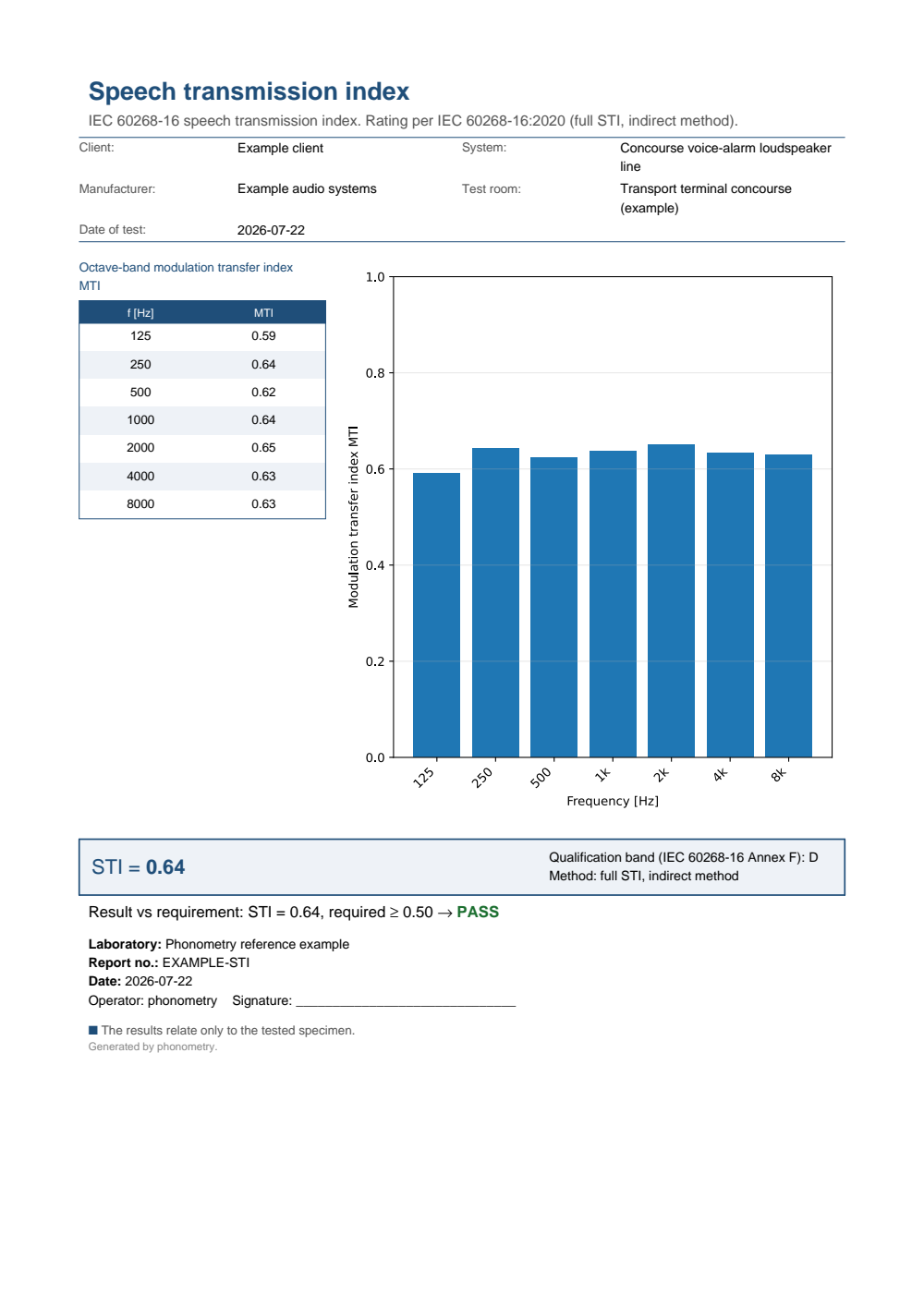
One-page speech-transmission-index fiche: a metadata header, an octave-band modulation transfer index table, the per-band MTI bars, the boxed STI = 0.64 single-number result with the Annex F qualification band and a PASS verdict against a 0.5 minimum.

Download the report (PDF)

Speech transmission index fiche (STIResult.report), STI with the Annex F band.

What this guide covers

Covered. IEC 60268-16:2020 (Edition 5) for the male speech option, the only one Edition 5 keeps: the modulation transfer function and the m to STI mapping (clauses A.5.2 to A.5.6), the full-STI indirect method from a measured impulse response via hearing.sti_from_impulse_response(), the direct STIPA method of Annex B via hearing.stipa_signal() and hearing.stipa(), the Ed.5 male test-signal spectrum of clause A.6.1, the level-dependent auditory masking and reception threshold corrections of Tables A.2 and A.3 (level= and ambient=), and the Annex F rating letters returned as STIResult.rating.

Not covered. The direct full-STI measurement (the 14-modulation-frequency test signal played and recorded through the real chain, per clause 6.3 and Table 3, recommended above when distortion is severe) is not implemented: only the STIPA direct signal (stipa_signal/stipa) and the indirect full-STI computation from an impulse response are available. The female speech option is not missing from the library: Edition 5 itself removed it (foreword, item d), so there is nothing left to implement.

See also

• Room Acoustics: the measured impulse response the indirect method consumes, and the open-plan metrics (ISO 3382-3) built on per-position STI.
• Speech Intelligibility Index: the audibility-based ANSI S3.5 index that complements the STI.
• Loudness and Sound Quality Metrics: loudness, sharpness, tonality and roughness of the received sound.
• Theory: the modulation-transfer derivation and the m ↔ STI mapping.
• API reference: hearing.sti.

References

• Houtgast, T., & Steeneken, H. J. M. (1985). A review of the MTF concept in room acoustics and its use for estimating speech intelligibility in auditoria. The Journal of the Acoustical Society of America, 77(3), 1069-1077. https://doi.org/10.1121/1.392224The modulation-transfer framework of section 1 and the m ↔ STI mapping the index is built on.
• International Electrotechnical Commission. (2020). Sound system equipment — Part 16: Objective rating of speech intelligibility by speech transmission index (IEC 60268-16:2020 (Edition 5)). The modulation transfer function and the m ↔ STI mapping, the STIPA test signal and direct method, the indirect method from the impulse response, auditory masking and the reception threshold (Tables A.2/A.3), the revised male speech spectrum (clause A.6.1) and the Annex F rating letters. Edition 4's normative PDF is the base and every Ed. 5 change is source-attributed, the only numeric delta being the revised male speech spectrum of clause A.6.1.