Time-frequency analysis

By José M. Requena Plens · Published Jul 21, 2026, updated Jul 26, 2026

Key references: Bendat & Piersol 2010 Harris 1978

A stationary spectrum hides everything that happens in time: a passing siren, an impact, a machine running up. This page covers the two time-frequency estimators of phonometry.metrology, both with the calibration discipline of the spectral-analysis page: the calibrated spectrogram (the short-time Fourier transform view of Bendat & Piersol Section 12.6.4.2, in absolute units - dB SPL for a signal in pascals) and the zoom FFT (Section 11.5.4), which computes the spectrum of a narrow band on an arbitrarily fine grid to separate tones closer than a practical full-band FFT bin. Where the levels page offers the fractional-octave-band spectrogram of a sound level meter, this one is its fine-band, constant-bandwidth counterpart.

1. The calibrated spectrogram

spectrogram splits the record into tapered (Hann by default), overlapped segments - exactly the segmentation of power_spectral_density - and keeps each segment’s one-sided periodogram as one column of the time-frequency display instead of averaging them. Because the calibration is the exact Welch-module scaling with no detrending, three identities hold:

a signal in pascals yields Pa²/Hz ('density') or Pa² ('spectrum') per cell, so 10·lg(power/p₀²) with 'spectrum' scaling reads a tone’s sound pressure level directly in any column it spans;
the column mean over time reproduces power_spectral_density bin by bin, with the same taper, overlap and scaling;
with a taper whose square overlap-adds to a constant (Hann at 75 % overlap), the time-integrated 'density' power equals the record’s time-domain energy exactly (Parseval plus the COLA identity - one of the conformance checks).

from phonometry import spectrogram

res = spectrogram(x, fs, nperseg=1024, overlap=0.75, scaling="spectrum")
print(res.power.shape)             # (frequencies, times)
print(res.time_resolution)         # T_B = nperseg/fs, in s
print(res.resolution_bandwidth)    # Be of the tapered segment, in Hz
res.plot()                         # dB image over the time-frequency plane

The segment length is the whole design decision: T_B = nperseg/fs of time resolution against Bₑ ≈ 1/T_B of frequency resolution, a product of one (Section 12.6.4.2). Long segments pin frequencies and smear transients; short segments do the opposite. And because each cell is a single unaveraged estimate, random data carries a per-cell normalized random error of 1 (Eq. 8.158 with nd = 1; Bendat & Piersol quote √2/1.25 ≈ 1.13 for the magnitude display) - the spectrogram is a tool for deterministic structure (tones, sweeps, transients), while the averaged Welch estimate is the low-variance tool for the stationary background.

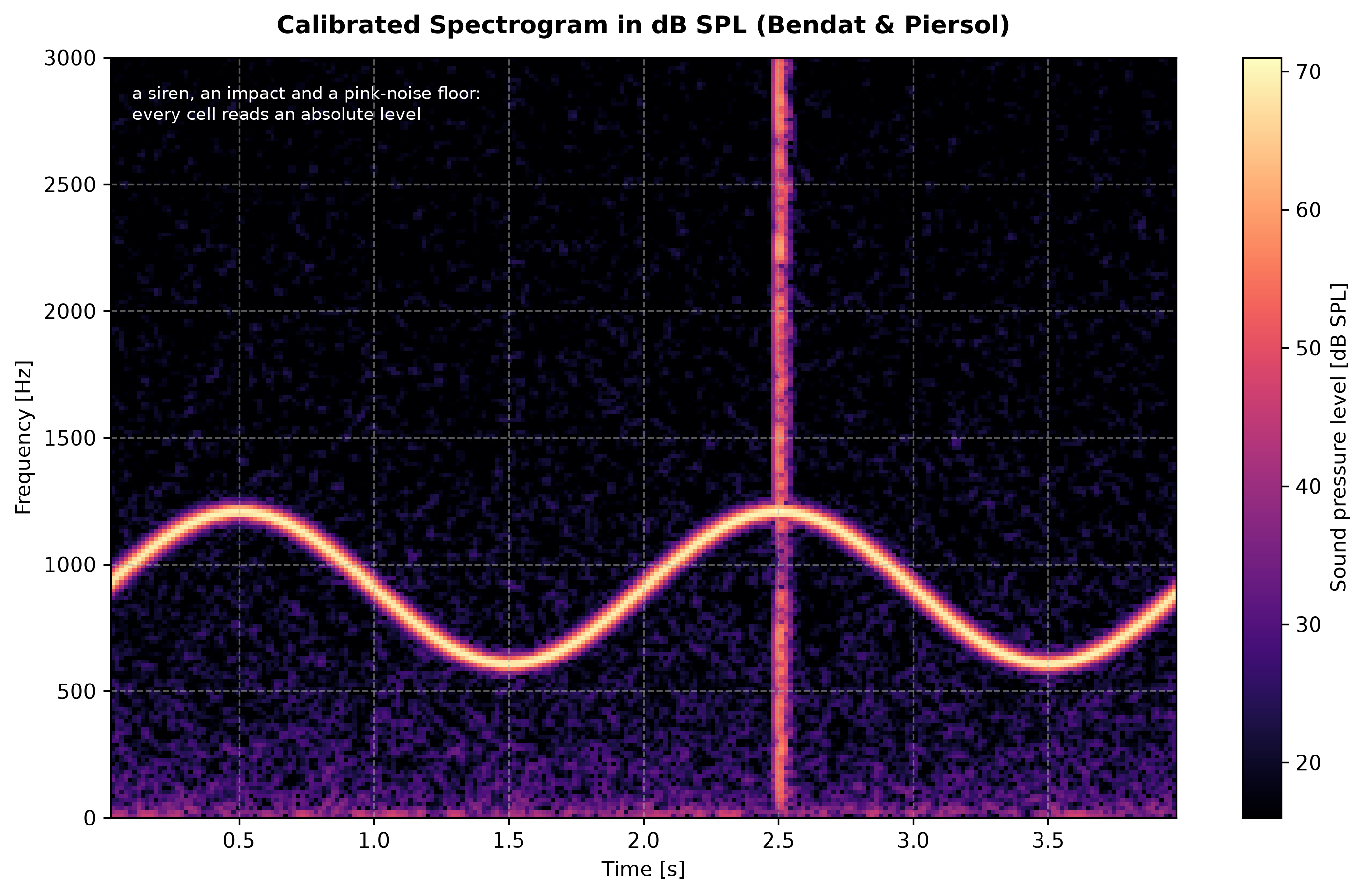
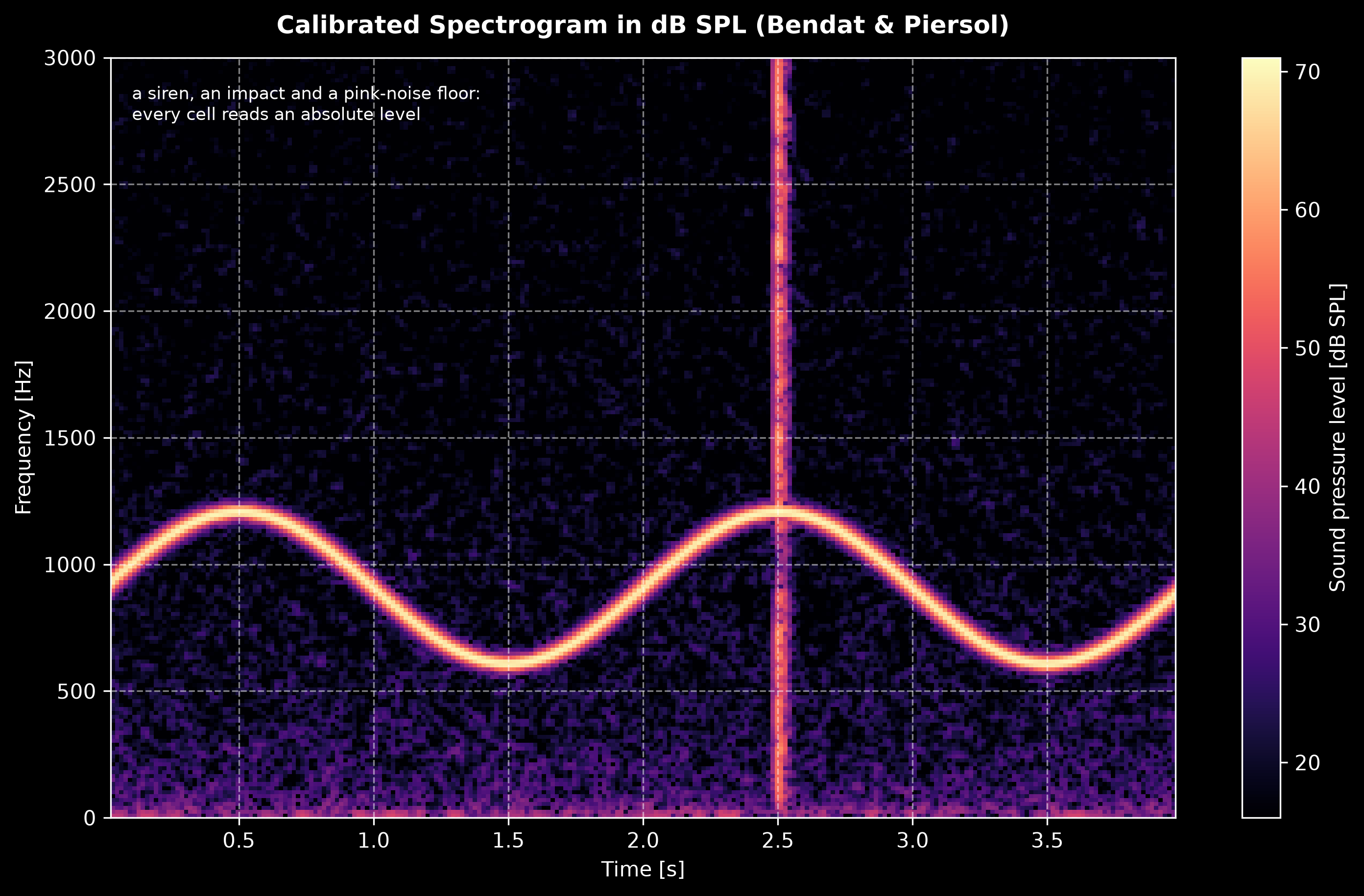
Calibrated spectrogram in dB SPL of a synthetic four-second outdoor scene: a siren sweeping sinusoidally between 600 and 1200 hertz traces a bright oscillating ridge at 70 decibels, a broadband impact at two and a half seconds draws a vertical stripe, and a pink noise floor at 45 decibels fills the background, with the color bar reading absolute sound pressure level

Show the code for this figure

import matplotlib.pyplot as plt
import numpy as np
from phonometry import noise_signal, spectrogram

fs = 16000.0
t = np.arange(int(4.0 * fs)) / fs
p_ref = 2e-5

siren_rms = p_ref * 10.0 ** (70.0 / 20.0)          # 70 dB SPL siren
x = siren_rms * np.sqrt(2.0) * np.cos(
    2.0 * np.pi * 900.0 * t - 600.0 * np.cos(np.pi * t)
)
rng = np.random.default_rng(9)
n_imp = int(0.06 * fs)                              # impact at t = 2.5 s
x[int(2.5 * fs):int(2.5 * fs) + n_imp] += 0.4 * (
    rng.standard_normal(n_imp) * np.exp(-np.arange(n_imp) / (0.012 * fs))
)
x += noise_signal(fs, 4.0, color="pink",            # 45 dB SPL floor
                  rms=p_ref * 10.0 ** (45.0 / 20.0), seed=10)

res = spectrogram(x, fs, nperseg=1024, overlap=0.75, scaling="spectrum")
level = 10.0 * np.log10(res.power / p_ref**2)

fig, ax = plt.subplots(figsize=(10, 6))
img = ax.imshow(level, cmap="magma", vmin=level.max() - 55.0,
                vmax=level.max(), aspect="auto", origin="lower",
                extent=(res.times[0], res.times[-1], 0.0,
                        res.frequencies[-1]))
fig.colorbar(img, ax=ax, label="Sound pressure level [dB SPL]")
ax.set_ylim(0.0, 3000.0)
ax.set_xlabel("Time [s]")
ax.set_ylabel("Frequency [Hz]")
plt.show()

res.plot() draws the same display from the result directly (a single raster image, 80 dB below the strongest cell by default; pass vmin/vmax to change the range, or ax to draw into an existing panel).

2. Zoom FFT

Two tones 3 Hz apart - gear sidebands, twin machines, mains hum against a rotor harmonic - are invisible to a 1024-point FFT at 8192 Hz: its bins are 8 Hz wide. The classical analyzer solution is the zoom transform of Bendat & Piersol Section 11.5.4: bandpass the record, shift the band down to zero frequency by complex demodulation with exp(-j2πf₁t) (Eqs. 11.123-11.126), decimate by the bandwidth ratio and Fourier transform the decimated record (Eqs. 11.128-11.130), obtaining a fine bin spacing over the band without a giant FFT block (Eq. 11.127).

zoom_fft computes the exact single-pass digital equivalent - the chirp-Z evaluation of the tapered record’s DFT on the zoom grid - which yields the same DFT samples as the demodulate-decimate chain; the test suite pins the two against each other at machine precision. Amplitudes are calibrated per the taper’s coherent gain, so a sine of peak amplitude A on an analysis frequency reads amplitude = A and power = A²/2 exactly:

from phonometry import zoom_fft

res = zoom_fft(x, fs, 980.0, 1016.0)     # grid at the record resolution
print(res.bin_spacing)                   # fs/N by default
print(res.resolution_bandwidth)          # Be of the tapered record
peak = res.amplitude.argmax()
print(res.frequencies[peak], res.amplitude[peak])
res.plot()                               # power spectrum in dB over the band

One distinction matters and the result states it: the grid can be made arbitrarily fine (n_points), but the resolution - the ability to separate two tones - is set by the record length and taper, reported as resolution_bandwidth (Bₑ = fs·Σw²/(Σw)², i.e. 1/T untapered, 1.5/T for Hann). Zooming refines the sampling of the same underlying spectrum; only a longer record separates closer tones.

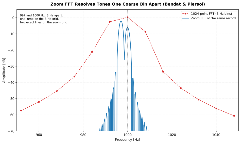
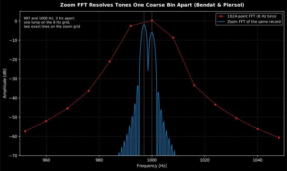
Zoom FFT of a one-second record containing tones at 997 and 1000 hertz: the coarse 1024-point FFT with 8 hertz bins shows a single broad lump, while the zoom FFT over 980 to 1016 hertz draws two separate mainlobes whose peaks sit exactly on the dotted true-tone frequencies

Show the code for this figure

import matplotlib.pyplot as plt
import numpy as np
from scipy import signal
from phonometry import zoom_fft

fs = 8192.0
t = np.arange(8192) / fs                 # 1 s record: 1 Hz resolution
x = (0.8 * np.cos(2.0 * np.pi * 997.0 * t)
     + 0.5 * np.cos(2.0 * np.pi * 1000.0 * t))

w = signal.get_window("hann", 1024)      # the coarse view: 8 Hz bins
coarse = 2.0 * np.abs(np.fft.rfft(x[:1024] * w)) / np.sum(w)
coarse_f = np.fft.rfftfreq(1024, 1.0 / fs)
band = (coarse_f >= 950.0) & (coarse_f <= 1050.0)

res = zoom_fft(x, fs, 980.0, 1016.0, n_points=145)   # 0.25 Hz grid

fig, ax = plt.subplots(figsize=(10, 6))
ax.plot(coarse_f[band], 20.0 * np.log10(coarse[band]), "o--",
        label="1024-point FFT (8 Hz bins)")
ax.plot(res.frequencies, 20.0 * np.log10(res.amplitude),
        label="Zoom FFT of the same record")
for f0 in (997.0, 1000.0):
    ax.axvline(f0, color="k", ls=":", lw=1.0, alpha=0.6)
ax.set_ylim(-70.0, 5.0)
ax.set_xlabel("Frequency [Hz]")
ax.set_ylabel("Amplitude [dB]")
ax.legend()
plt.show()

Relation to the rest of the library

The spectrogram shares its taper, segmentation and scaling with power_spectral_density, so the two are mutually consistent bin by bin; the octave-band spectrogram of OctaveFilterBank.spectrogram is the constant-percentage-bandwidth counterpart with sound-level-meter ballistics; and for tracking a single component’s frequency in time, the Hilbert instantaneous frequency of envelope complements the STFT ridge.

What this guide covers

Covered. Bendat & Piersol’s calibrated spectrogram (Section 12.6.4.2): tapered, overlapped STFT segments kept as separate time columns instead of averaged, implemented by spectrogram with the exact Welch-module scaling and the Eq. 8.158 random error of an unaveraged cell. The zoom FFT of Section 11.5.4 (Eqs. 11.122-11.130): band-limited, arbitrarily fine-grid spectra computed as the chirp-Z equivalent of the book’s demodulate-decimate-DFT chain, implemented by zoom_fft. Both share the Harris (1978) window catalogue behind the segment taper.

Not covered. This is the constant-bandwidth, STFT-based family only. The constant-percentage-bandwidth, sound-level-meter counterpart is OctaveFilterBank.spectrogram on the Levels page. Tracking a single component’s instantaneous frequency over time is the Hilbert envelope of envelope, on the Correlation and delay page, not this one. As with the spectral-analysis page, this implements Bendat & Piersol’s estimators, not a certification standard.

References

Bendat, J. S., & Piersol, A. G. (2010). Random data: Analysis and measurement procedures (4th ed.). Wiley. https://doi.org/10.1002/9781118032428Section 12.6.4.2 (spectrograms and their random errors), Section 11.5.4 (zoom transform procedures, Eqs. 11.122-11.130) and Sections 8.5.1/8.5.4 (resolution bandwidth and the statistical errors of unaveraged estimates). ISBN 978-0-470-24877-5.
Harris, F. J. (1978). On the use of windows for harmonic analysis with the discrete Fourier transform. Proceedings of the IEEE 66(1), 51-83. https://doi.org/10.1109/PROC.1978.10837The taper catalogue behind the segment window: main-lobe width versus sidelobe leakage, the trade-off that sets what a spectrogram column can resolve at a given segment length.

Created and maintained byJosé Manuel Requena Plens· GitHub· PyPI· All projects