2D FDTD wave simulation

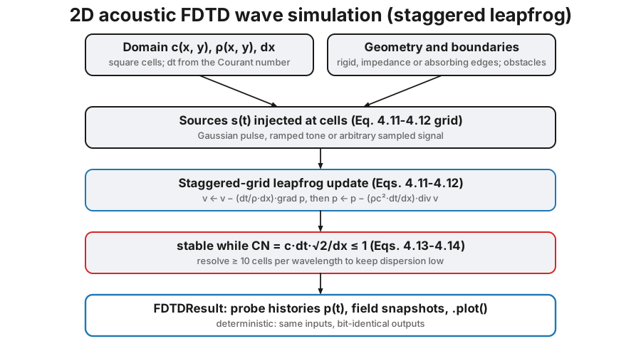
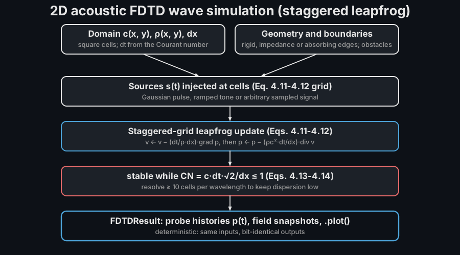
Most of phonometry predicts a number: a level, a reverberation time, a transmission loss. The simulation domain computes the wave field itself: fdtd_simulation integrates the linear acoustic equations on a 2D grid with the finite-difference time-domain (FDTD) method, so reflection, diffraction, interference, refraction through inhomogeneous media and modal behaviour all emerge from first principles instead of being modelled term by term. The implementation follows the reference formulation for outdoor sound of Attenborough & Van Renterghem, Predicting Outdoor Sound (2nd ed., CRC Press 2021), chapter 4: the staggered-in-place, staggered-in-time pressure-velocity scheme (Eqs. 4.11-4.12), the Courant stability condition (Eqs. 4.13-4.14), rigid boundaries as zero normal face velocity (Eq. 4.32) and the frequency-independent real-impedance boundary (Eqs. 4.33-4.35).

The solver is deterministic by design: float64 arithmetic, no random numbers and single-threaded numpy stepping, so the same inputs produce bit-identical outputs on the same platform. It is the engine behind the FDTD animations of this documentation, promoted to a public API with sources, pressure probes, rasterised obstacles, per-side boundary conditions and a frozen result object.

1. The scheme: a wave equation on a grid

In a non-moving medium the linearised equations of fluid dynamics reduce to a first-order system in the acoustic pressure p and particle velocity v (Attenborough & Van Renterghem Eqs. 4.3-4.4):

$$\frac{\partial p}{\partial t}+\rho c^2\nabla \cdot \mathbf{v}=0,\frac{\partial \mathbf{v}}{\partial t}+\frac{1}{\rho }\nabla p=0.$$

FDTD discretises both on a staggered grid (the acoustic analogue of the Yee cell): pressure lives at cell centres and each velocity component on the cell faces, half a cell away, and the two fields leapfrog in time, half a time step apart (Eqs. 4.11-4.12). Evaluating each spatial gradient exactly where the other field needs it gives a fourfold accuracy gain over a collocated grid (Eq. 4.9 vs 4.10) and allows in-place updates. Because only interior faces are stored, the domain edge is a perfectly rigid wall (zero normal velocity, Eq. 4.32) unless another boundary is requested.

The explicit scheme is stable only while a wavefront crosses at most one cell per time step. With square cells the Courant number (Eq. 4.13) is

$$\mathrm{CN}=c\Delta t\sqrt{\frac{1}{\Delta x^2}+\frac{1}{\Delta y^2}}=\frac{c\Delta t\sqrt{2}}{\Delta x}\le 1,$$

and fdtd_simulation derives the time step from the cfl parameter (the Courant number, default 0.6) and the largest sound speed in the map; values outside (0, 1) are rejected because the scheme is unconditionally meaningless beyond the bound (Eq. 4.14).

from phonometry import simulation

# A 3.0 x 2.0 m air domain: 300 x 200 cells of 1 cm.
res = simulation.fdtd_simulation(
    343.0, 0.01, 2.0e-3, shape=(200, 300),
    sources=[simulation.GaussianPulse(ix=60, iy=100, width=3.0e-4)],
    probes=[(200, 100)],
)
print(res.size)                  # (3.0, 2.0)  metres
print(round(res.dt * 1e6, 2))    # 12.37  microseconds (CN = 0.6)
res.plot()                       # probe pressure histories (figure in §3)

The grid is index-based: cell (ix, iy) has its centre at ((ix + 0.5) * dx, (iy + 0.5) * dx) metres, with rows plotted downward (the imshow convention), so a position in metres maps to ix = round(x / dx - 0.5).

2. Sources, probes, obstacles and boundaries

Three source types inject a soft source (an additive pressure contribution that does not scatter passing waves) at a grid cell: GaussianPulse (a broadband pulse of temporal half-width width), CWSource (a sine tone faded in with a raised-cosine ramp so its onset does not splash a broadband transient) and SignalSource (an arbitrary sampled waveform, linearly interpolated onto the simulation time steps). Probes record the pressure at their cell every time step into the result.

Geometry is rasterised: obstacle_mask marks rigid cells, and every face touching a masked cell is closed (Eq. 4.32 again), so walls, barriers and scatterers of any shape are just boolean arrays. Each domain side can carry its own boundary condition:

• "rigid" (default): a perfect reflector, R = +1.
• "absorbing": a sponge layer of absorbing_layer_cells cells whose absorption rate ramps quadratically, emulating an open boundary (the simple precursor of the perfectly matched layers of section 4.2.3).
• a real specific impedance Z in Pa·s/m (a scalar or one value per edge cell): the locally reacting boundary of Eqs. 4.33-4.35, updated implicitly, with the normal-incidence reflection coefficient R = (Z - ρc)/(Z + ρc); Z = ρc is anechoic.

The stepping engine FDTD2D is public too: it exposes step(), run(), the field arrays and the energy, for callers that need frame-by-frame access (the documentation animations use it directly). A plane pulse launched down a duct against an impedance edge reproduces the textbook reflection coefficient:

import numpy as np
from phonometry import simulation

rho, c, dx = 1.2, 343.0, 0.01
sim = simulation.FDTD2D(c, dx, rho=rho, shape=(3, 1200),
                        edge_impedance={"right": 3.0 * rho * c})
x = (np.arange(1200) + 0.5) * dx
sim.p[:] = np.exp(-(((x - 6.0) / 0.15) ** 2))[None, :]   # plane pulse

trace = []
for _ in range(int(round(0.032 / sim.dt))):
    sim.step()
    trace.append(sim.p[1, 900])
trace = np.asarray(trace)
t = (np.arange(trace.size) + 1) * sim.dt
t_return = 6.0 / c + 3.0 / c                  # via the wall, back to x = 9 m
incident = trace[t < t_return - 0.001].max()
echo = trace[t > t_return]
print(round(float(echo[np.abs(echo).argmax()] / incident), 2))  # 0.5
# (Z - rho c)/(Z + rho c) = (3 - 1)/(3 + 1) = +0.5

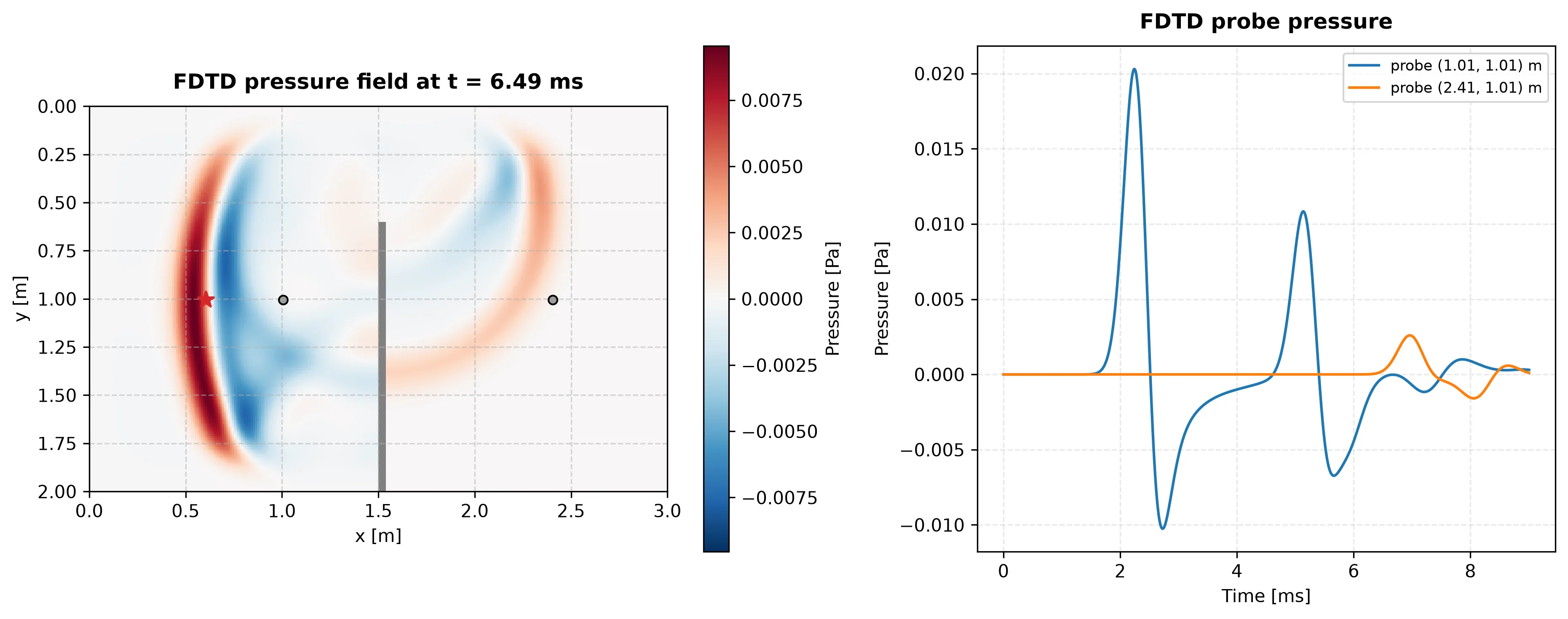
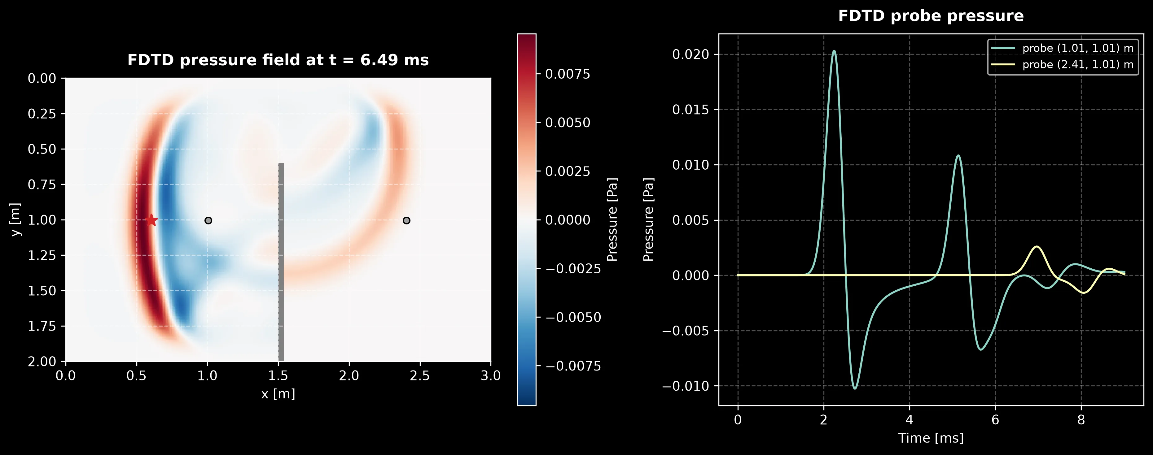
3. When to use it, and the 2D limits

FDTD earns its cost when the geometry drives the physics: diffraction around a barrier or through an opening, interference of direct and reflected paths, scattering from obstacles, modal behaviour of odd-shaped enclosures, refraction through a sound-speed gradient. One run captures all frequencies at once (a pulse excites the whole band; one FFT of a probe yields the spectrum), where a frequency-domain method needs one solve per frequency.

Show the code for this figure

import numpy as np
import matplotlib.pyplot as plt
from phonometry import simulation

# A 3.0 x 2.0 m free field (absorbing edges) with a thin rigid barrier:
# probe A sees the direct pulse plus the barrier reflection, probe B sits
# in the shadow and only receives the wave diffracted around the edge.
mask = np.zeros((200, 300), dtype=bool)
mask[60:, 150:154] = True
res = simulation.fdtd_simulation(
    343.0, 0.01, 9.0e-3, shape=(200, 300),
    sources=[simulation.GaussianPulse(ix=60, iy=100, width=3.0e-4)],
    probes=[(100, 100), (240, 100)],
    obstacle_mask=mask,
    boundaries="absorbing", absorbing_layer_cells=30,
    snapshot_every=75,
)

fig, (ax_f, ax_p) = plt.subplots(
    1, 2, figsize=(12.5, 5.0), gridspec_kw={"width_ratios": [1.25, 1.0]})
res.plot(kind="snapshot", frame=7, ax=ax_f)
res.plot(ax=ax_p)
plt.tight_layout()
plt.show()

Conversely, when a validated closed form exists (statistical reverberation, ISO 9613-2 outdoor attenuation, image sources in a rectangular room) the closed form is thousands of times cheaper: this solver is the cross-check and the demonstrator, not the replacement. The oracle works both ways; a rigid-box run reproduces the analytic room modes:

import numpy as np
from phonometry import simulation

lx, ly, dx = 1.0, 0.7, 0.02
nx, ny = round(lx / dx), round(ly / dx)
res = simulation.fdtd_simulation(
    343.0, dx, 0.35, shape=(ny, nx),
    sources=[simulation.GaussianPulse(ix=7, iy=5, width=2.0e-4)],
    probes=[(nx - 4, ny - 3)],
)
p = res.pressures[0]
spec = np.abs(np.fft.rfft(p * np.hanning(p.size), n=8 * p.size))
freqs = np.fft.rfftfreq(8 * p.size, res.dt)
sel = (freqs > 250) & (freqs < 350)
print(round(0.5 * 343.0 * float(np.hypot(1 / lx, 1 / ly)), 1))  # 299.1  exact (1,1) mode
print(round(float(freqs[sel][np.argmax(spec[sel])]), 1))        # 298.9  measured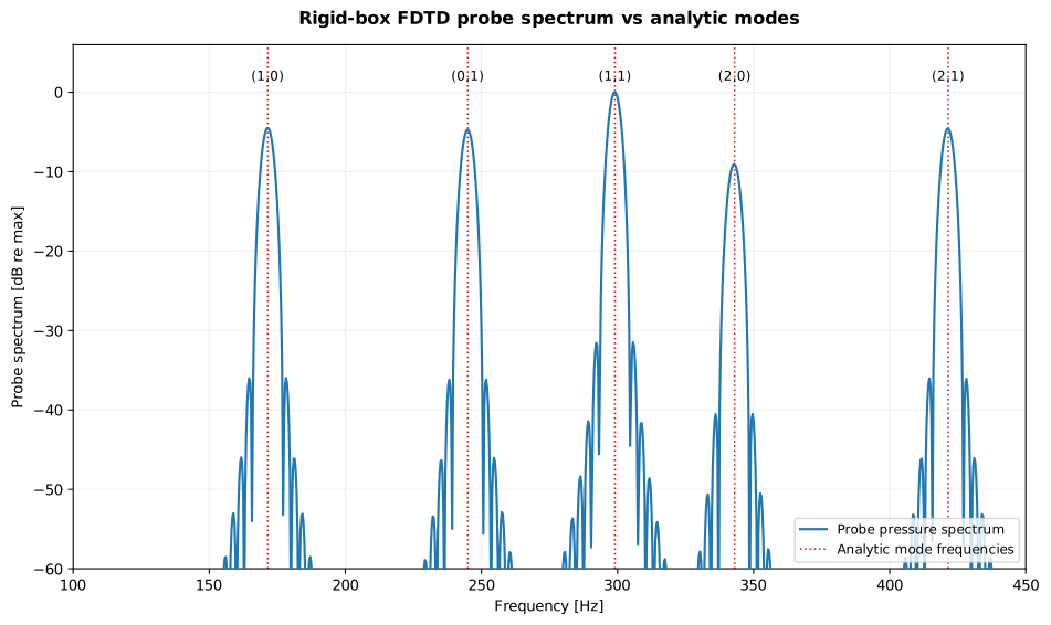

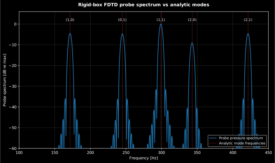
The probe spectrum of the rigid-box run peaks exactly on the analytic mode frequencies $f=(c/2)\sqrt{(n_x/L_x{)}^2+(n_y/L_y{)}^2}$ (Kuttruff 6e, Ch. 3). The barely visible leftward offset of the highest peaks is the numerical dispersion of §4: short wavelengths propagate slightly slow on the grid, so the modelled resonances under-read by a fraction of a percent.

Show the code for this figure

import numpy as np
import matplotlib.pyplot as plt
from phonometry import simulation

lx, ly, dx, c = 1.0, 0.7, 0.02, 343.0
nx, ny = round(lx / dx), round(ly / dx)
res = simulation.fdtd_simulation(
    c, dx, 0.35, shape=(ny, nx),
    sources=[simulation.GaussianPulse(ix=7, iy=5, width=2.0e-4)],
    probes=[(nx - 4, ny - 3)],
)

# One line: the raw probe pressure history the spectrum is computed from.
res.plot()
plt.show()

# The mode check: probe spectrum against the analytic rigid-room modes.
p = res.pressures[0]
spec = np.abs(np.fft.rfft(p * np.hanning(p.size), n=8 * p.size))
freqs = np.fft.rfftfreq(8 * p.size, res.dt)
sel = (freqs >= 100) & (freqs <= 450)
fig, ax = plt.subplots()
ax.plot(freqs[sel], 20 * np.log10(spec[sel] / spec[sel].max()))
for mx, my in [(1, 0), (0, 1), (1, 1), (2, 0), (2, 1)]:
    ax.axvline(0.5 * c * np.hypot(mx / lx, my / ly), ls=":", color="tab:red")
ax.set(xlabel="Frequency [Hz]", ylabel="Probe spectrum [dB re max]",
       ylim=(-60, 6))
plt.show()

The domain is two-dimensional, and that changes the physics, not just the cost. A 2D point source is physically an infinite line source: its amplitude spreads cylindrically as 1/sqrt(r) (3.0 dB per doubling of distance) instead of the spherical 1/r (6.0 dB) of a 3D point source, and the 2D impulse response trails a wake behind the wavefront instead of passing cleanly. Interference and diffraction patterns are faithful; absolute levels and decay rates are not those of a 3D room. Treat 2D runs as cross-sections and demonstrations, and validate any 3D-quantitative claim against a closed form or a 3D solver.

4. Numerical dispersion and accuracy

The discrete grid propagates each frequency at a slightly wrong speed: short wavelengths lag, so a sharp pulse develops a ripple tail and resonances shift slightly. This numerical dispersion is the discrete counterpart of Eq. 4.15; on the axes of a square grid the scheme’s dispersion relation is

$$\sin \left(\frac{\omega \Delta t}{2}\right)=\frac{c\Delta t}{\Delta x}\sin \left(\frac{k\Delta x}{2}\right),$$

with a leading-order relative frequency error of magnitude (1 - S^2) (k dx)^2 / 24 along the grid axes (the modelled frequency under-reads, so the signed error is negative), where S = c dt / dx; the error is largest exactly on-axis and vanishes along the cell diagonal at the Courant limit CN = 1. The practical rule is to resolve at least 10 cells per shortest wavelength, dx <= c_min / (10 f_max) with the smallest sound speed of the domain: at exactly 10 cells the small-Courant bound (k dx)^2 / 24 evaluates to about 1.6 %, reduced by the 1 - S^2 factor to about 1.4 % at the default cfl = 0.6 (in a heterogeneous domain the time step follows the fastest cells, so slower regions run at a lower local Courant number and sit nearer the 1.6 % bound), and every finer-resolved or off-axis component is more accurate. With dx = 1 cm the 10-cell point in air sits at roughly 3.4 kHz, and halving dx quarters the error (the scheme is second order, and the validation suite measures that observed order under grid refinement). The tests pin the solver to analytic oracles: box and duct eigenfrequencies, free-field arrival times and cylindrical decay, the rigid-wall image echo, the impedance reflection coefficient above and the dispersion relation itself.

The frozen FDTDResult carries the time axis, the per-probe pressure histories, the probe positions in metres, the grid metadata, the sources, the optional field snapshots with their times and the obstacle mask; its .plot() draws the probe histories, and .plot(kind="snapshot") renders one recorded field with the geometry overlaid.

What this guide covers

Covered. The staggered pressure-velocity FDTD scheme of Attenborough & Van Renterghem, chapter 4: the governing equations (Eqs. 4.3-4.4), the leapfrog update (Eqs. 4.11-4.12), the Courant stability condition (Eqs. 4.13-4.14), the rigid boundary (Eq. 4.32) and the frequency-independent real-impedance boundary (Eqs. 4.33-4.35), exposed through fdtd_simulation/ FDTD2D with GaussianPulse, CWSource and SignalSource sources, pressure probes and a rasterised obstacle_mask. Validated against closed-form oracles: the rigid-room normal modes (Kuttruff §3), free-field arrival times and cylindrical 2D decay, the rigid-wall image echo, the impedance reflection coefficient and the dispersion relation of §4, with the measured convergence order matching the scheme’s second-order design.

Not covered. The solver is two-dimensional only: it models a line source in cross-section (cylindrical 1/sqrt(r) spreading), not the spherical 1/r spreading of a 3D point source, so absolute levels and decay rates are not those of a 3D room. The open boundary is the quadratic-ramp absorbing layer described as “the simple precursor” of a true perfectly matched layer, not a PML itself. The governing equations assume a non-moving medium, so wind or flow advection is not modelled, and the only impedance boundary is the frequency-independent real one of Eqs. 4.33-4.35.

See also

• Conformance report: two of the closed-form validation anchors of §4 run there.
• API reference: simulation.fdtd.

Quick answers

How do I choose the FDTD grid spacing?

Resolve at least 10 cells per shortest wavelength, dx <= c_min / (10 f_max), using the smallest sound speed in the domain. At exactly 10 cells the on-axis dispersion error bound is about 1.6 %, reduced to about 1.4 % at the default cfl = 0.6, and halving dx quarters the error (the scheme is second order). With dx = 1 cm the 10-cell point in air sits at roughly 3.4 kHz.

What Courant number keeps an FDTD simulation stable?

The explicit scheme is stable only while a wavefront crosses at most one cell per time step. With square cells the Courant number is $\mathrm{CN}=c\Delta t\sqrt{2}/\Delta x\le 1$ (Attenborough & Van Renterghem Eq. 4.13). fdtd_simulation derives the time step from the cfl parameter (the Courant number, default 0.6) and the largest sound speed in the map, rejecting values outside $(0,1)$.

Can I trust the absolute levels from a 2D FDTD run?

No. A 2D point source is physically an infinite line source: its amplitude spreads cylindrically as 1/sqrt(r), 3.0 dB per doubling of distance, instead of the spherical 1/r (6.0 dB per doubling) of a 3D point source. Interference and diffraction patterns are faithful, but absolute levels and decay rates are not those of a 3D room; validate any 3D-quantitative claim against a closed form or a 3D solver.

References

• Attenborough, K., & Van Renterghem, T. (2021). Predicting outdoor sound (2nd ed.). CRC Press. https://doi.org/10.1201/9780429470806Chapter 4: the pressure-velocity FDTD reference model implemented here, from the governing equations (4.3-4.4) and the staggered leapfrog update (4.11-4.12) through the Courant condition (4.13-4.14), the phase-error analysis (4.15) and the rigid and finite-impedance boundary conditions (4.32-4.35). The module implements this textbook numerical method rather than a measurement standard, with this chapter as the citable reference formulation.
• Kuttruff, H. (2016). Room acoustics (6th ed.). CRC Press. https://doi.org/10.1201/9781315372150Section 3.5 places time-domain wave-based methods among the numerical approaches to the wave equation in enclosures, and chapter 3 gives the rigid-room normal modes used as the analytic oracle.