Multichannel and Performance

Most real measurement sessions produce more than one channel: the two ears of a dummy head, the microphone pair of an intensity probe, the several positions of a room survey, the capsules of a beamforming array. The convention for all of them is one array of shape (channels, samples) processed in a single call: every function runs along the last (time) axis and preserves the leading channel axis, so each row is analyzed exactly as if it were the only one.

That per-channel guarantee is normative, not just convenient. The band filters applied to each row are the IEC 61260-1 designs and the weightings and detector ballistics are the IEC 61672-1 ones, unchanged from the single-channel path; the vectorization batches the arithmetic across rows (one filter design, one SciPy call) and never mixes them. This is the textbook procedure for multiple data records (Bendat & Piersol 2010, §10.4.2): analyze each record individually first, and compute anything joint as a separate, explicit step.

Use this page when your channels are parallel recordings on the same clock and you want per-channel spectra or levels. When the question is between channels (what is the delay from A to B, how much of B is explained by A), that is cross-channel analysis: see Correlation and delay and Multiple and partial coherence, the implementations of the Bendat & Piersol cross-correlation and multiple-input models.

A stereo analysis in one call

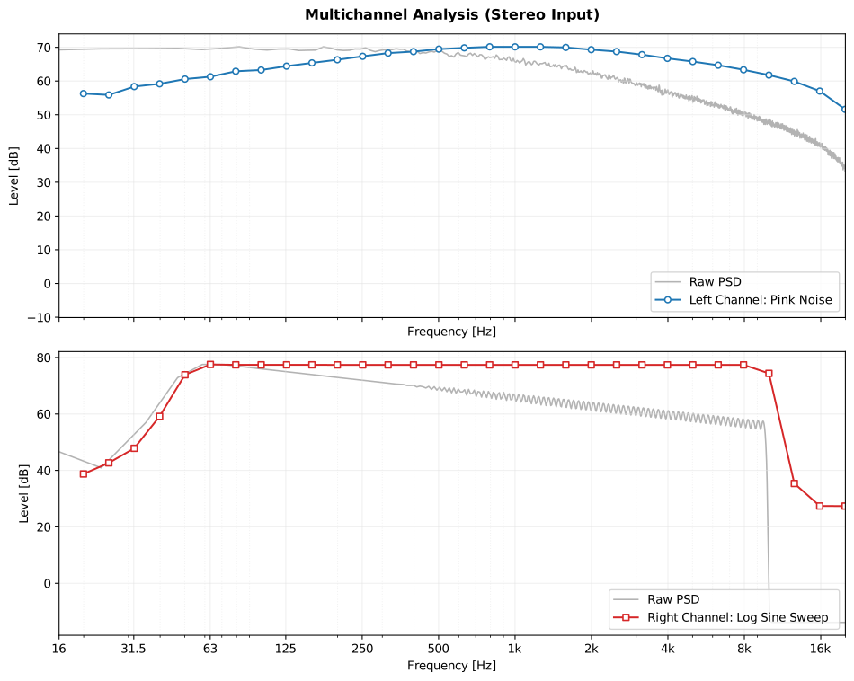
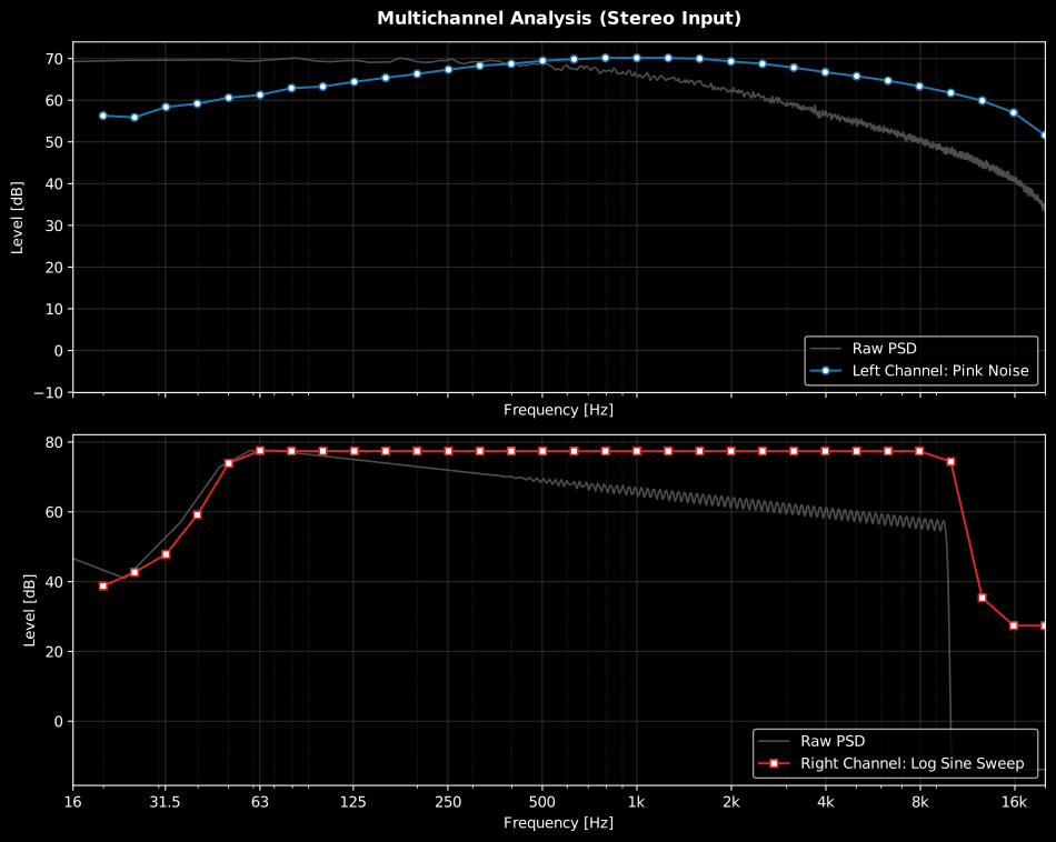
Simultaneous analysis of a Stereo signal: Left Channel (Pink Noise) vs Right Channel (Log Sine Sweep).

Show the code for this figure

import matplotlib.pyplot as plt
import numpy as np
from scipy.signal import chirp
from phonometry import metrology

# Stereo test signal: pink noise left, logarithmic sine sweep right
fs, duration = 48000, 5
t = np.linspace(0, duration, fs * duration, endpoint=False)
rng = np.random.default_rng(42)
spec = np.fft.rfft(rng.standard_normal(t.size))
spec[1:] /= np.sqrt(np.arange(1, spec.size))   # 1/f shaping: pink noise
left = np.fft.irfft(spec, t.size)
right = chirp(t, f0=50, t1=duration, f1=10000, method="logarithmic")

x = np.stack([left, right])                    # (2, n_samples)
spl, freq = metrology.octave_filter(x, fs, fraction=3, limits=[20, 20000])

fig, axes = plt.subplots(2, 1, figsize=(9, 7), sharex=True)
for ax, levels, name in zip(axes, spl, ["Left: pink noise", "Right: log sweep"]):
    ax.semilogx(freq, levels, marker="o", label=name)
    ax.set_ylabel("Level [dB]")
    ax.grid(True, which="both", alpha=0.3)
    ax.legend()
axes[-1].set_xlabel("Frequency [Hz]")
plt.show()

The convention is consistent across the whole library: time is always the last axis. This applies to octave_filter, OctaveFilterBank, weighting_filter, time_weighting, leq, laeq, ln_levels and spectrogram.

import numpy as np
from phonometry import metrology

# Two calibrated channels in Pa so the guide runs standalone
fs = 48000
t = np.arange(fs) / fs
left = 0.2 * np.sin(2 * np.pi * 1000 * t)
right = 0.1 * np.sin(2 * np.pi * 500 * t)

stereo = np.stack([left, right])          # (2, n_samples)
spl, freq = metrology.octave_filter(stereo, fs, fraction=3)
# spl has shape (2, n_bands): one row per channel

Accepted shapes, at a glance

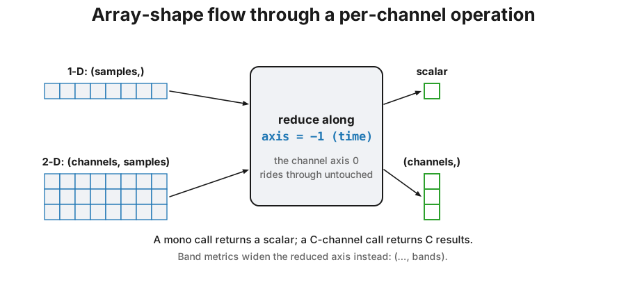
Input	Interpreted as	Typical output
(n,) 1D array	one channel	scalar level / (bands,)
(ch, n) 2D array	ch channels, n samples each	(ch,) levels / (ch, bands)
list of floats	one channel (converted)	as 1D
(ch, n) into spectrogram	multichannel STFT-style	(ch, bands, frames)

Everything vectorizes across the leading channel axis: one filter design is applied to all channels in a single SciPy call, so 8 channels cost far less than 8 separate runs. Convention: channels first, like most DSP code (soundfile returns (n, ch): transpose with x.T).

Per-channel semantics

Multichannel processing is strictly per channel: nothing is ever mixed, summed or averaged across the channel axis. Three consequences worth spelling out:

• Combining channels is your decision. Levels come back one per channel. If you need an array-average level (for instance the position-averaged levels of the room-acoustics standards), combine energies yourself: 10 * np.log10(np.mean(10 ** (spl / 10), axis=0)), never the arithmetic mean of the dB values (see Levels for why).
• One calibration_factor means one sensitivity. The scalar factor multiplies every channel, which is correct only if all channels share the same sensitivity. For an array of microphones with individual calibrations, scale the rows first, x * factors[:, None], and leave calibration_factor at 1.
• Stateful classes keep one state per channel. In block processing the state array matches the channel count and a change of channel count resets it; see Block Processing.

Performance: Vectorization and caching

OctaveFilterBank is the tool for repeated or streaming analysis: one bank designs its filters once and applies them to every frame, and NumPy broadcasting covers all channels of a frame in one filtering call per band, with no Python loop over channels.

import numpy as np
from phonometry import metrology

# Two calibrated channels in Pa so the guide runs standalone
fs = 48000
t = np.arange(fs) / fs
left = 0.2 * np.sin(2 * np.pi * 1000 * t)
right = 0.1 * np.sin(2 * np.pi * 500 * t)
stereo = np.stack([left, right])          # (2, n_samples)

bank = metrology.OctaveFilterBank(fs=48000, fraction=3, filter_type='butter')

# Access computed properties
# bank.freq (center), bank.freq_d (lower), bank.freq_u (upper), bank.sos (coefficients)

# Process multiple signals efficiently
stream = [stereo]                 # your sequence of multichannel frames
for frame in stream:
    # detrend=True (default) removes DC offset to improve low-freq accuracy
    spl, freq = bank.filter(frame, detrend=True)

Additional performance notes:

• Design cache: octave_filter() reuses filter bank designs across calls with identical parameters (LRU cache, 32 entries), so calling it in a loop does not redesign the bank each time. OctaveFilterBank gives you explicit control over the design lifetime.
• Multirate decimation: low-frequency bands are filtered at a decimated rate, which is both faster and numerically more stable (see Theory).
• Optional numba: the impulse time weighting kernel is JIT-compiled when numba is installed (pip install phonometry[perf]).

What this guide covers

Covered. IEC 61260-1:2014 and IEC 61672-1:2013 as far as they constrain each row of a (channels, samples) array: the band filters, weightings and detector ballistics applied per channel are the unchanged single-channel designs, and multichannel support adds no normative content of its own. The convention itself follows Bendat & Piersol’s procedure for multiple data records (Section 10.4.2): analyze each record individually first, and treat anything joint as a separate, explicit step.

Not covered. Cross-channel questions, such as the delay between two channels or how much of one channel a second one explains, are deliberately left out: octave_filter, weighting_filter and time_weighting never mix or combine rows. See Correlation and delay and Multiple and partial coherence for the cross-channel tools built on Bendat & Piersol’s cross-correlation and multiple-input models.

See also

• Correlation and delay: the cross-channel time-domain questions (delay, alignment) the per-channel path deliberately leaves to you.
• Multiple and partial coherence: which of several correlated channels actually drives a response (Bendat & Piersol Ch. 7).
• Block Processing: the streaming counterpart, with one filter state per channel.
• Levels: the per-channel level metrics, and why dB values are combined energetically.
• API reference: phonometry and metrology.core.

References

• Bendat, J. S., & Piersol, A. G. (2010). Random data: Analysis and measurement procedures (4th ed.). Wiley. https://doi.org/10.1002/9781118032428Section 10.4.2 (the procedure for analyzing multiple data records: individual per-record analysis first, joint cross-record analysis as a separate, deliberate step) and Chapter 7 (the multiple-input/output models that joint step leads to). ISBN 978-0-470-24877-5.
• International Electrotechnical Commission. (2013). Electroacoustics — Sound level meters — Part 1: Specifications (IEC 61672-1:2013). The weighting and time-integration semantics applied per channel, exactly as the single-channel standard prescribes.
• International Electrotechnical Commission. (2014). Electroacoustics — Octave-band and fractional-octave-band filters — Part 1: Specifications (IEC 61260-1:2014). The band definitions each channel is filtered with; the multichannel path batches them unchanged. Multichannel support adds no normative content of its own: each channel is filtered exactly as the single-channel standard prescribes, and the vectorization only batches the computation across the channel axis.