Installed structure-borne sound (EN 12354-5)

EN 12354-5:2009 predicts the sound pressure level in a receiving room caused by building service equipment (pumps, fans, lifts, water installations) that injects structure-borne sound into the building. It closes the structural-vibroacoustics chain: the source is described by its characteristic structure-borne sound power level L_Ws,c, derived from the EN 15657 reception-plate measurement through the Formula (15)/(17) conversion and a mobility correction (not the raw plate-injected level; see EN 15657); the source and receiver point mobilities set how much power is actually coupled into the structure, and the building transmission carries it to the receiving room. The Annex I mobility correction installed_power_from_reception_plate refers the characteristic reception-plate level L_Ws,n to the actual receiver, L_Ws,inst = L_Ws,n + 10 lg(Y_∞,i / Y_∞,rec) with Y_∞,rec = 5·10⁻⁶ m/(N·s); with the source mobility instead it yields L_Ws,c (Annex I.3, Table I.8).

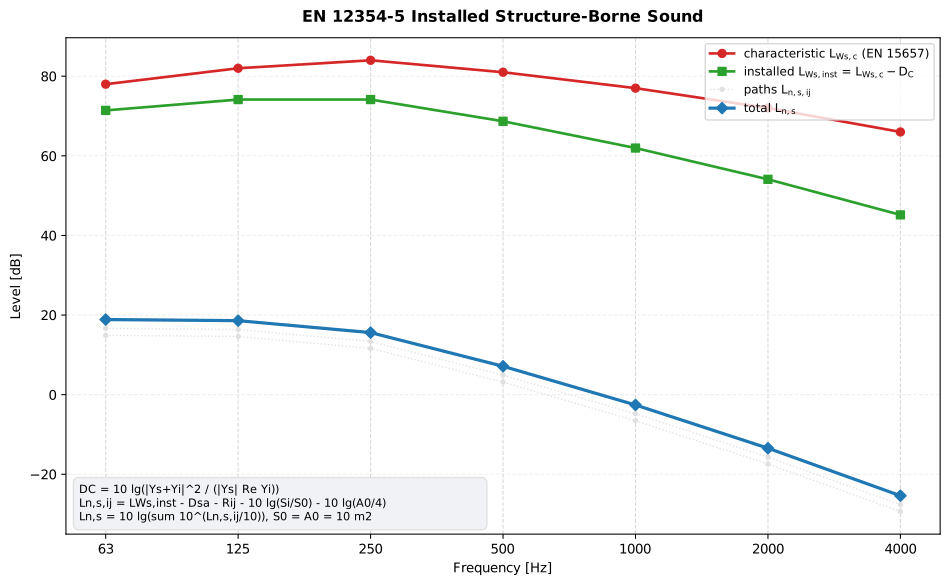
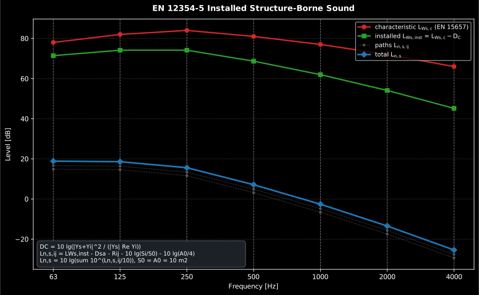
Show the code for this figure

import matplotlib.pyplot as plt
import numpy as np
from phonometry import building

# EN 15657 characteristic source power and illustrative point mobilities.
bands = np.array([63.0, 125.0, 250.0, 500.0, 1000.0, 2000.0, 4000.0])
lws_c = np.array([78.0, 82.0, 84.0, 81.0, 77.0, 72.0, 66.0])
ys = (2e-4 + 1e-4j) * (bands / 250.0)        # source mobility
yi = (3e-5 + 1e-5j) * np.ones_like(bands)    # receiver mobility
dc = np.array([float(building.coupling_term(a, b)) for a, b in zip(ys, yi)])

# Two transmission paths: the excited floor and a flanking wall.
paths = [
    {"adjustment_term": 6.0, "element_area": 12.0,
     "flanking_reduction_index": np.linspace(44.0, 62.0, 7)},
    {"adjustment_term": 7.0, "element_area": 9.0,
     "flanking_reduction_index": np.linspace(46.0, 64.0, 7)},
]
res = building.installed_source_prediction(lws_c, dc, paths, frequencies=bands)
res.plot()   # characteristic and installed power, per-path levels and the total
plt.show()

1. Coupling and installed power

Only part of the characteristic power is injected into the supporting element; the loss is the coupling term D_C (always positive), set for a point excitation by the source mobility Y_s and the receiver mobility Y_i (Formula 19b):

$$D_{C,i}=10\lg \frac{|Y_s+Y_i{|}^2}{|Y_s|\mathrm{Re}\{Y_i\}},$$

which reduces to 10 lg(|Y_s|/Re{Y_i}) for a force source (high source mobility, Formula 19c) and to −10 lg(|Y_s|·Re{Z_i}) for a velocity source (low source mobility, Formula 19d); an elastic support adds its transfer mobility Y_k inside the modulus (Formula 19e). The installed power level is then (Formula 18b) L_Ws,inst = L_Ws,c − D_C.

The physics behind D_C is the classical power input of a point-excited plate: only the real part of the receiver’s driving-point mobility absorbs power, and the mismatch between Y_s and Y_i decides how much of the source’s capability ever enters the structure (Hopkins 2007, Section 2.8). The mobilities themselves come from the mechanical-mobility chain: measured per ISO 7626, or from the infinite-plate closed forms of panel theory when no measurement exists. A pump on a concrete slab is the textbook force source: its casing mobility is orders of magnitude above the slab’s, so D_C collapses to Formula 19c and the injected power no longer depends on the receiver at all.

from phonometry import building

# A near-force source (Y_s >> Y_i) on a concrete floor:
dc = building.coupling_term(2e-4 + 1e-4j, 3e-5 + 1e-5j)
print(round(float(dc), 2))                                          # ~8.5 dB
print(round(float(building.installed_structure_borne_power_level(82.0, dc)), 1))  # installed L_Ws

2. Transmission to the receiving room

EN 12354 parts 1 and 2 handle rooms excited through the air and by the standard tapping machine; part 5 covers the sources that shake the building directly: pumps, fans, lifts, whirlpool baths, cisterns and the pipework that ties them into walls and floors. Once the installed power is in the structure, several elements radiate into the receiving room: the excited element itself and every element the vibration reaches across the junctions. Each excited-element/radiating-element pair i→j is a transmission path with its own adjustment term and flanking index:

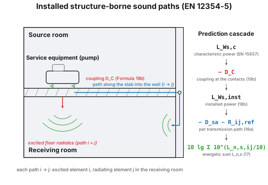
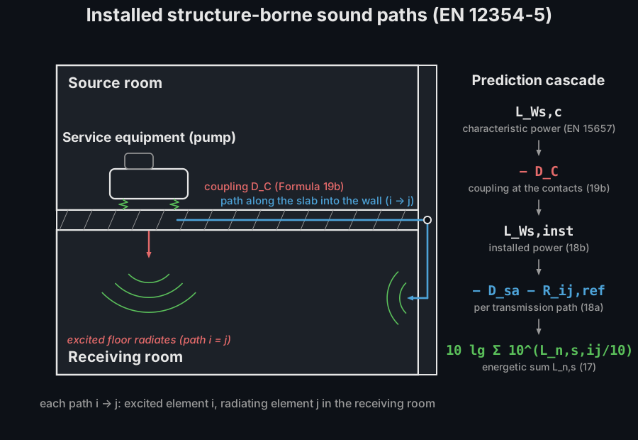
Each transmission path i→j gives a normalised sound pressure level from the installed power, the structure-to-airborne adjustment term D_sa, the flanking sound reduction index R_ij,ref (EN 12354-1) and the element area (Formula 18a):

$$L_{n,s,ij}=L_{Ws,\mathrm{inst},i}-D_{sa,i}-R_{ij,\mathrm{ref}}-10\lg \frac{S_i}{S_0}-10\lg \frac{A_0}{4},$$

with S₀ = A₀ = 10 m², and the paths combine energetically (Formula 17):

import numpy as np
from phonometry import building

bands = np.array([250.0, 500.0, 1000.0])
res = building.installed_source_prediction(
    characteristic_power_level=np.array([80.0, 82.0, 78.0]),
    coupling_term=np.array([9.0, 10.0, 11.0]),
    paths=[
        {"adjustment_term": 5.0,
         "flanking_reduction_index": np.array([50.0, 52.0, 55.0]), "element_area": 12.0},
        {"adjustment_term": 6.0,
         "flanking_reduction_index": np.array([52.0, 54.0, 57.0]), "element_area": 8.0},
    ],
    frequencies=bands,
)
print(np.round(res.total_level, 1))      # total L_n,s per band
print(round(res.overall_level, 1))       # band-summed level [dB]

res.plot()   # the per-path and total L_n,s cascade, as in the figure above (needs matplotlib)

The InstalledSourceResult carries the per-path levels, the total per band, the installed power level and .overall_level, and its .plot() draws the whole cascade.

3. The prediction report (.report())

A prediction ends as a document. The InstalledSourceResult exposes a .report() method that writes a one-page PDF fiche, clearly labelled a prediction, not a measurement: a prediction-basis line naming EN 12354-5:2009, an optional metadata header (client, source equipment, receiving room, instrumentation, climate, date), a per-band table (nominal octave/one-third-octave frequency, the installed structure-borne power level $L_{Ws,inst}$, each transmission path’s normalised SPL $L_{n,s,ij}$ and the combined total $L_{n,s}$), the per-path and total $L_{n,s}(f)$ spectra, and a boxed band-summed total $L_{n,s}$ (dB) with the installed power total and the path count.

The metadata is supplied through a ReportMetadata, whose applicable fields here are the source equipment (specimen), the receiving room (test_room), the client, the instrumentation and the footer identity (laboratory, operator, report_id, notes). Supplying requirement adds a PASS/FAIL verdict against a declared upper limit on the overall $L_{n,s}$ (less is better). verbose=True adds one column per transmission path (up to five); otherwise only the installed power and the combined total are shown. language="es" renders the Spanish fiche with comma decimals. The basis strip states Formulae 18a/17 and the prediction disclaimer.

import numpy as np
from phonometry import ReportMetadata, installed_source_prediction

bands = np.array([63, 125, 250, 500, 1000, 2000], float)
lwc = np.array([84.4, 82.5, 69.9, 67.6, 61.6, 49.9])   # characteristic power [dB]
dsa = np.array([-13.6, -17.3, -17.4, -20.0, -26.9, -32.9])
paths = [
    {"adjustment_term": dsa,
     "flanking_reduction_index": np.array([43.0, 46, 50.2, 54.7, 64.6, 73]),
     "element_area": 12.8},
    {"adjustment_term": dsa,
     "flanking_reduction_index": np.array([37.0, 41.2, 35.9, 37.7, 49, 57.8]),
     "element_area": 12.8},
]
res = installed_source_prediction(lwc, 16.2, paths, frequencies=bands)

res.report(
    "installed_structure_borne.pdf",
    metadata=ReportMetadata(
        client="Example dwelling refurbishment",
        specimen="WC flushing cistern (wall-fixed)",
        test_room="Receiving room: adjacent bedroom",
        report_id="EXAMPLE-12354-5",
        requirement=45.0,
    ),
)   # overall L_n,s ~ 43 dB -> declared limit 45 dB: PASS

The example fiche is regenerated with make reports and kept rendered in the repository; click the preview to open the PDF.

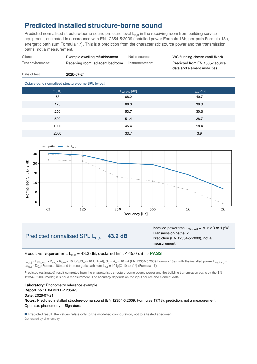
One-page EN 12354-5:2009 installed structure-borne sound prediction fiche, clearly labelled a prediction and not a measurement: a header with the client, the source equipment, the receiving room and the identity, the octave-band table (63 Hz to 2 kHz) of the installed structure-borne power level L_Ws,inst, the two flanking paths' normalised SPL L_n,s,ij and the combined total L_n,s, the per-path and total L_n,s(f) spectra, and the boxed band-summed total L_n,s with the installed power total and the path count, closed by a basis strip stating Formulae 18a/17 and the prediction disclaimer, with a PASS verdict against the declared 45 dB limit.

Download the report (PDF)

Installed structure-borne prediction fiche (InstalledSourceResult.report), an EN 12354-5 estimate of the normalised structure-borne SPL in the receiving room.

What this guide covers

Covered. EN 12354-5:2009: the coupling term D_C (clause 4.4.3, Formulae 19b-e, with its force-source and velocity-source limits) via coupling_term, the installed power level L_Ws,inst = L_Ws,c − D_C (Formula 18b) via installed_structure_borne_power_level, and the per-path normalised sound pressure level and its energetic total (Formulae 18a, 17) via installed_source_prediction. Validated against the standard’s own Annex I worked examples, the whirlpool bath (I.2) and the flushing cistern (I.3), within the ±0.15 dB rounding of the printed intermediates.

Not covered. The Annex D and F default-value tables for the structure- to-airborne adjustment term D_sa and the flanking reduction index R_ij,ref are not implemented; both are inputs you supply from measurement, EN 12354-1 or the standard’s own annexes. Only the 2009 edition is implemented, not the 2023 revision.

See also

• Structure-borne sound power of equipment (EN 15657): the reception-plate characterisation that supplies L_Ws,c and the source mobility this prediction consumes.
• Mechanical mobility and the FRF family (ISO 7626-1): the measured Y_s and Y_i behind the coupling term.
• Bending-wave transmission at plate junctions: the junction physics that carries the installed power to the flanking radiators.
• Predicting Sound Insulation (EN 12354): the airborne and impact members of the same prediction family.
• API reference: building.installed_structure_borne.

References

• Cremer, L., Heckl, M., & Petersson, B. A. T. (2005). Structure-borne sound: Structural vibrations and sound radiation at audio frequencies (3rd ed.). Springer. https://doi.org/10.1007/b137728The source-receiver mobility coupling and the structure-borne transmission across junctions behind the coupling term and the path model. ISBN 978-3-540-22696-3.
• European Committee for Standardization. (2009). Building acoustics — Estimation of acoustic performance of buildings from the performance of elements — Part 5: Sound levels due to service equipment (EN 12354-5:2009). The coupling term (clause 4.4.3, Formulae 19a-19e), the installed structure-borne power level (Formula 18b), the structure-to-airborne adjustment term (clause 4.4.4, Formulae 20a/20b), and the normalised sound pressure level per path and its energetic combination (Formulae 18a, 17). Conformance is anchored on the coupling-term force-source limit and the standard's own Annex I worked examples: the whirlpool bath of I.2 (Table I.6a: mobility correction and path 11) and the flushing cistern of I.3 (Tables I.8/I.9: source conversion, all four transmission paths, the Formula 17 total and its 29 dB(A) closure), within the ±0.15 dB rounding of the printed one-decimal intermediates. D_sa and R_ij,ref are inputs (from measurement / EN 12354-1 / Annexes D and F). The linked catalogue record is the BSI Knowledge page for BS EN 12354-5:2009; since revised as EN 12354-5:2023 (https://knowledge.bsigroup.com/products/building-acoustics-estimation-of-acoustic-performance-of-buildings-from-the-performance-of-elements-sounds-levels-due-to-the-service-equipment).
• Hopkins, C. (2007). Sound insulation. Butterworth-Heinemann. https://doi.org/10.4324/9780080550473Section 2.8 (driving-point impedance and mobility): the power a mechanical source injects into a plate through the source and receiver mobilities, the building-acoustics reading of the clause 4.4.3 coupling term. ISBN 978-0-7506-6526-1.