Bending-wave transmission at plate junctions

When a bending wave travelling on a wall or floor reaches a rigid junction with another plate, part of its energy is reflected and part is transmitted into the connected plates. The wave approach of Cremer et al. (1973), tabulated by Craik (1981, 1996) and collected in Hopkins (2007, Section 5.2.1.3), gives the transmission coefficient in closed form for the four most common junctions of thin, homogeneous, isotropic plates: the X, T, L and in-line junctions. Modelling the junction as a simply supported (pinned) massless beam forces an incident bending wave to generate only reflected and transmitted bending waves, with no conversion to in-plane waves, and the resulting coefficients are independent of frequency. That is what makes them convenient closed-form inputs for statistical energy analysis (SEA) and for the EN 12354 flanking-transmission model, where they feed the coupling loss factor etaij and the vibration reduction index Kij.

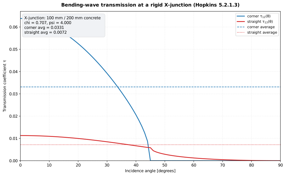
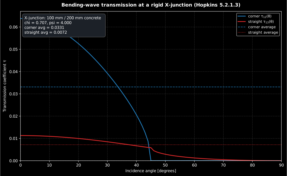
Show the code for this figure

import matplotlib.pyplot as plt
from phonometry import junction_transmission

# X-junction between a 100 mm and a 200 mm concrete plate (cL = 3200 m/s).
res = junction_transmission("X", 0.1, 3200.0, 240.0, 0.2, 3200.0, 480.0)
res.plot()  # tau(theta) for the corner and straight paths, with averages
plt.show()

1. Wave parameters chi and psi

With plate i of thickness h_i, quasi-longitudinal wave speed cL_i and surface density rho_s,i, the whole family of coefficients depends on just two dimensionless ratios (Cremer et al. 1973):

chi = kB2 / kB1 = (rho_s2 B1 / (rho_s1 B2))**0.25 = sqrt(h1 cL1 / (h2 cL2)) = sqrt(fc2 / fc1)
psi = B2 kB2**2 / (B1 kB1**2) = (h2 cL2 rho_s2) / (h1 cL1 rho_s1) = (rho_s2 fc1) / (rho_s1 fc2)

chi is the ratio of the plates’ bending wavenumbers (equivalently the square root of their critical-frequency ratio) and sets the total-internal-reflection cut-off angle theta_co = arcsin(chi); psi is the ratio of their bending-moment mobilities. For identical plates both are 1.

from phonometry import junction_wave_parameters

chi, psi = junction_wave_parameters(0.1, 3200.0, 240.0, 0.2, 3200.0, 480.0)
#  -> (sqrt(0.5), 4.0)

2. Corner and straight-section coefficients

For an incident wave on plate 1, transmission around the corner (into the perpendicular plate 2) is tau12(theta) (Eq. 5.12), and transmission across the straight section (into the collinear plate 3, X- and T-junction (1) only) is tau13(theta) (Eq. 5.13). The corner coefficient is zero beyond the cut-off, tau12(theta) = 0 for chi < sin(theta). The junction constants J1, J2, J3 select the geometry:

Junction	J1	J2	J3
X	1	1	1
T-junction (1)	2	0.5	0.5
T-junction (2)	2	2	—
L	4	1	—

The straight section is undefined for the T-junction (2) and the L-junction.

import numpy as np
from phonometry import (
    corner_transmission_coefficient,
    straight_transmission_coefficient,
)

theta = np.radians(np.linspace(0.0, 90.0, 91))
tau12 = corner_transmission_coefficient(theta, chi, psi, "X")
tau13 = straight_transmission_coefficient(theta, chi, psi, "X")

3. Diffuse-field angular average

In a diffuse vibration field every angle of incidence is equally probable and the incident intensity carries a cos(theta) obliquity factor, so the average transmission coefficient is tau_bar_ij = integral 0..pi/2 of tau_ij(theta) cos(theta) d(theta) (Eq. 5.6). For identical plates the algebra collapses to exact fractions that serve as the library’s first-principles oracle:

• X-junction corner and straight: tau_ij(theta) = cos**2(theta) / 8, so tau_bar_ij = 1/12;
• L-junction corner: tau_ij(theta) = cos**2(theta) / 2, so tau_bar_ij = 1/3;
• in-line junction: tau12(0 deg) = 1 (a continuous plate transmits fully).

from phonometry import angular_average_transmission_coefficient

angular_average_transmission_coefficient(1.0, 1.0, "X", section="corner")  # 1/12
angular_average_transmission_coefficient(1.0, 1.0, "L", section="corner")  # 1/3

The two directions obey the SEA consistency relationship (Eq. 5.7), tau_bar_12 = chi * tau_bar_21, so only one direction needs to be computed.

4. Coupling loss factor and vibration reduction index

The angular average is the bridge to the two junction descriptors used in SEA-based building models: the coupling loss factor (Eq. 2.154) etaij = cg_i L_ij tau_ij / (2 pi**2 f S_i) and the wave-approach vibration reduction index (Eq. 5.116) Kij = 10 lg(1 / tau_ij) + 5 lg(fc_j / f_ref) with f_ref = 1000 Hz and fc_j the critical frequency of the receiving plate. Combined with the Eq. 5.7 reciprocity this form is symmetric, Kij = Kji, as EN 12354 requires of the junction descriptor. For the identical 100 mm concrete X-junction (fc ~= 203 Hz), Kij = 10 lg 12 + 5 lg(203 / 1000) ~= 7.3 dB.

from phonometry import (coupling_loss_factor, junction_transmission,
                        wave_vibration_reduction_index)

eta = coupling_loss_factor(1.0 / 12.0, group_velocity=200.0,
                           junction_length=4.0, frequency=500.0, plate_area=10.0)
res = junction_transmission("X", 0.1, 3200.0, 240.0, 0.1, 3200.0, 240.0)
kij = wave_vibration_reduction_index(res.corner_average,
                                     res.critical_frequency2)  # 7.33 dB
kij = res.corner_reduction_index  # the same, precomputed on the result

res.plot()   # tau(theta) for this junction's corner and straight paths (needs matplotlib)

The junction descriptor is a design quantity: sweeping the receiving plate’s thickness shows how much a mass change at the junction buys. The corner paths stiffen quickly with a heavier receiving plate, while the straight (in-line) path of the X-junction rises fastest of all, since the perpendicular plates increasingly pin the junction line:

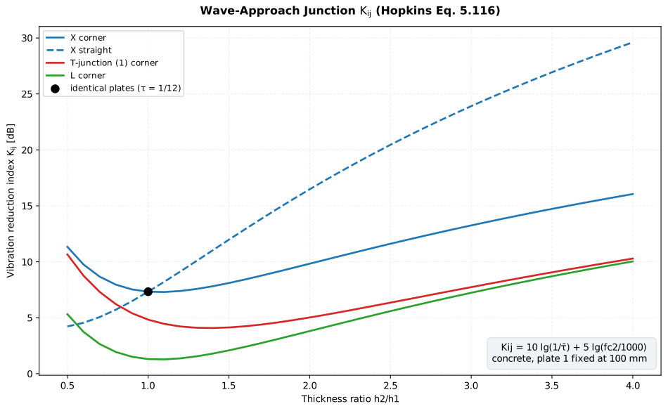
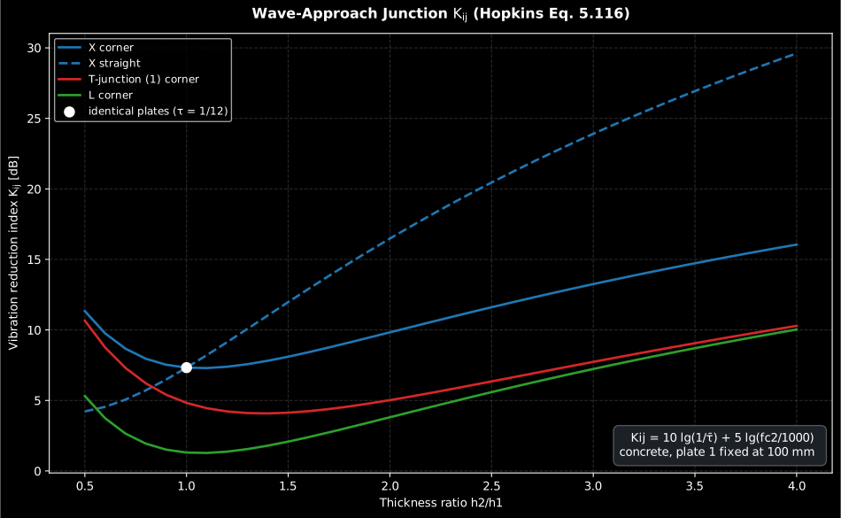
Show the code for this figure

import matplotlib.pyplot as plt
import numpy as np
from phonometry import junction_transmission, wave_vibration_reduction_index

# Concrete plates (cL = 3200 m/s, rho = 2400 kg/m3): plate 1 fixed at
# 100 mm, plate 2 swept from 50 mm to 400 mm.
h1, cl, rho = 0.1, 3200.0, 2400.0
ratios = np.linspace(0.5, 4.0, 36)
kij_corner = []
for ratio in ratios:
    h2 = h1 * float(ratio)
    res = junction_transmission("X", h1, cl, rho * h1, h2, cl, rho * h2)
    kij_corner.append(res.corner_reduction_index)

fig, ax = plt.subplots()
ax.plot(ratios, kij_corner, label="X corner")
ax.set_xlabel("Thickness ratio h2/h1")
ax.set_ylabel("Vibration reduction index Kij [dB]")
ax.set_title("Wave-approach junction Kij (Hopkins Eq. 5.116)")
ax.legend()
plt.show()

5. Worked example: feeding Kij into EN 12354

The number this page predicts is exactly what the EN 12354-1 flanking model consumes. Take the 100 mm / 200 mm concrete X-junction from the figure at the top: its corner path gives K12 = 9.8 dB. Handing that to flanking_element in place of a tabulated Annex E value prices the junction’s three flanking paths and their effect on the apparent rating:

from phonometry import building, junction_transmission

# The 100 mm / 200 mm concrete X-junction of the opening figure:
res = junction_transmission("X", 0.1, 3200.0, 240.0, 0.2, 3200.0, 480.0)
k12 = res.corner_reduction_index                     # 9.8 dB (corner path)

# Feed it to the EN 12354-1 simplified model as this junction's Kij:
ff, df, fd = building.flanking_element(
    label="floor", r_flanking=49.0, r_separating=57.0,
    k_ff=k12, k_fd=k12, k_df=k12, separating_area=11.5, coupling_length=4.5)
pred = building.predicted_airborne_insulation(r_direct=57.0,
                                              flanking_paths=[ff, df, fd])
print(round(pred.r_prime_w, 1))                      # 55.4  (Rw 57 direct)
print(pred.dominant.label, round(pred.dominant.fraction, 2))   # Dd 0.68

One junction with a moderate Kij already trims 1.6 dB off the direct $R_w=57$ dB; a full building repeats this for every junction, which is the EN 12354 prediction guide.

The measured, EN 12354 counterpart of Kij (from the direction-averaged velocity level difference) is the separate flanking-transmission vibration_reduction_index; this page is the closed-form predicted value from the wave approach.

What this guide covers

Covered. The frequency-independent, rigid-junction transmission coefficients of Cremer, Heckl & Ungar (1973), tabulated by Craik (1981/1996) and collected in Hopkins (2007, Section 5.2.1.3), for the X, T, L and in-line junctions of thin, homogeneous, isotropic plates: the wave parameters $\chi$/$\psi$, the corner and straight-section coefficients ${\tau }_{12}(\theta )$/${\tau }_{13}(\theta )$, their diffuse-field angular average, the SEA coupling loss factor and the wave-approach vibration reduction index $K_{ij}$, via junction_wave_parameters, corner_transmission_coefficient, straight_transmission_coefficient, angular_average_transmission_coefficient, coupling_loss_factor, wave_vibration_reduction_index and junction_transmission.

Not covered. This predicted $K_{ij}$ is a closed-form idealisation for a rigid, simply supported junction, not a measurement: the measured, empirical $K_{ij}$ from a direction-averaged velocity level difference (ISO 10848) is the separate vibration_reduction_index of the Laboratory Insulation Measurement guide. The straight-section coefficient ${\tau }_{13}$ is undefined for the T-junction (2) and L-junction geometries, which have no collinear third plate, so only the corner path applies there.

See also

• Predicting Sound Insulation (EN 12354): the flanking model that consumes Kij junction by junction.
• Laboratory Insulation Measurement: the ISO 10848 measurement of Kij from velocity level differences, the empirical counterpart of this page’s closed forms.
• Structure-borne sound power of equipment (EN 15657): the source power that these junction transmissions carry through a building.
• Mechanical mobility and the FRF family (ISO 7626-1): the plate mobilities behind the wave parameters.
• API reference: vibration.junction_transmission.

References

• Craik, R. J. M. (1996). Sound transmission through buildings using statistical energy analysis. Gower. The SEA treatment of building sound transmission with the tabulated bending-wave transmission coefficients for X, T, L and in-line junctions used here (Eqs 5.12/5.13). ISBN 978-0-566-07572-5.
• Cremer, L., Heckl, M., & Ungar, E. E. (1973). Structure-borne sound: Structural vibrations and sound radiation at audio frequencies (1st ed.). Springer. https://doi.org/10.1007/978-3-662-10118-6The original derivation of the wave parameters chi and psi (Eqs 5.10/5.11 in Hopkins) and the in-line normal-incidence transmission coefficient. ISBN 978-3-540-06002-4.
• Hopkins, C. (2007). Sound insulation. Butterworth-Heinemann. https://doi.org/10.4324/9780080550473Section 5.2.1.3 collects the rigid X, T, L and in-line junction coefficients, the angular average (Eq. 5.6), the SEA consistency relationship (Eq. 5.7), the coupling loss factor (Eq. 2.154) and the wave-approach Kij (Eq. 5.116) implemented on this page. ISBN 978-0-7506-6526-1.