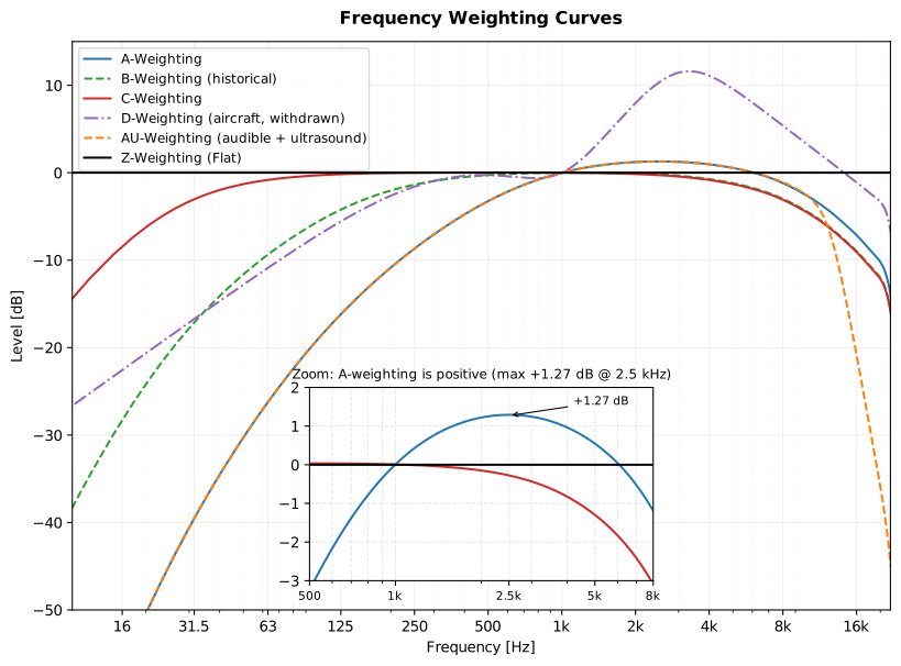
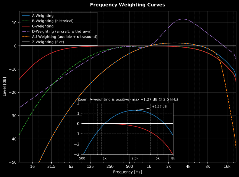
Frequency Weighting (A, B, C, D, G, AU, Z)

Frequency weighting curves simulate the human ear’s sensitivity. A, C and Z are specified by IEC 61672-1:2013; the infrasound G curve is specified by ISO 7196:1995. Three more curves round out the family: the historical B (ANSI S1.4-1983), the withdrawn aircraft-noise D (IEC 537) and AU (IEC 61012) for audible sound in the presence of ultrasound (section 4).

Show the code for this figure

import matplotlib.pyplot as plt
import numpy as np
from phonometry import metrology

# Measure each curve's response: weight a centered unit impulse and take
# its spectrum (1 s buffer -> 1 Hz frequency resolution).
fs = 48000
impulse = np.zeros(fs)
impulse[fs // 2] = 1.0
freqs = np.fft.rfftfreq(fs, 1 / fs)

fig, ax = plt.subplots(figsize=(9, 5))
for curve in ("A", "B", "C", "D", "AU", "Z"):
    spectrum = np.fft.rfft(metrology.weighting_filter(impulse, fs, curve=curve))
    ax.semilogx(freqs[1:], 20 * np.log10(np.abs(spectrum[1:]) + np.finfo(float).eps),
                label=curve)
ax.set(xlim=(10, 20000), ylim=(-80, 15),
       xlabel="Frequency [Hz]", ylabel="Response [dB]")
ax.grid(True, which="both", alpha=0.3)
ax.legend()
plt.show()

• A-Weighting (A): Standard for environmental noise (IEC 61672-1).
• C-Weighting (C): Used for peak sound pressure and high-level noise.
• Z-Weighting (Z): Zero weighting, completely flat response.
• G-Weighting (G): Infrasound weighting per ISO 7196 (see below).
• B-Weighting (B): Historical middle curve of ANSI S1.4-1983 (section 4).
• D-Weighting (D): Aircraft-noise weighting of the withdrawn IEC 537 (section 4).
• AU-Weighting (AU): A-weighting with the IEC 61012 ultrasound cutoff (section 4).

How do I apply A-weighting to a signal in Python?

Call metrology.weighting_filter(recording, fs, curve='A') on a calibrated signal. It returns the A-weighted time signal, filtered with the pole-zero design of IEC 61672-1:2013 within class 1 tolerances, so metrology.leq() on the output is the $L_{Aeq}$. The same function applies C, Z, B, D, AU and the infrasound G weighting through curve.

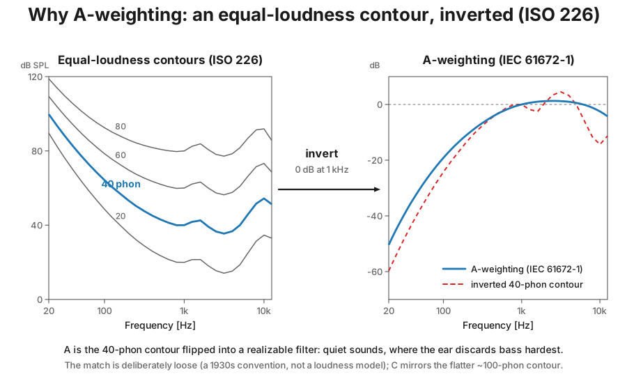
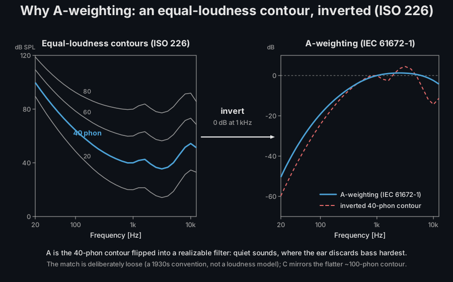
1. Where the curves come from

The A and C curves are inverted equal-loudness contours, frozen into filters: A approximates the inverse of the historic 40-phon contour (quiet levels, where the ear discards bass most aggressively) and C the flatter ~100-phon one (loud levels). IEC 61672-1:2013 (Annex E) defines both analytically from four corner frequencies:

$$f_1=20.599\text{Hz},f_2=107.653\text{Hz},f_3=737.862\text{Hz},f_4=12194.217\text{Hz}$$

C is a band-pass with double poles at $f_1$ and $f_4$ (2 zeros at the origin); A adds the $f_2$ and $f_3$ poles (4 zeros), which is why it keeps falling through the low-mids. Both are normalized to exactly 0 dB at 1 kHz. Z is the absence of weighting. The full pole/zero derivation is in the Theory page.

A short history: A, B, C and Z

The chain runs from Fletcher and Munson’s 1933 equal-loudness measurements to the first American sound level meter standard (1936), which gave meters switchable responses so the reading could approximate loudness at different levels: A from the 40-phon contour for quiet sounds, B from the ~70-phon contour for moderate ones, and a flat response for loud ones (the C curve proper, mirroring the flatter ~100-phon contour, arrived with the 1944 revision). Switching curves by level died in practice (readings jumped at the switch points, and field measurements became incomparable), but A survived alone: decades of hearing-damage and community-annoyance data had been collected with it, and it correlates with both about as well as far more elaborate metrics. IEC 61672-1 (first edition 2002) finished the cleanup: B was dropped, A and C were kept with tightened tolerances, and Z was introduced to replace the vaguely specified “linear” of older meters, which varied by manufacturer. The B curve (and the aircraft-noise D curve that met the same fate) remains available for historical data; see section 4.

When C − A matters

Because A discards bass and C keeps it, the difference $L_{Ceq}-L_{Aeq}$ is a one-number indicator of low-frequency content:

• Below about 10 dB: an ordinary broadband spectrum; the A-weighted level rates it fairly.
• Around 15 to 20 dB or more: the energy is concentrated at low frequencies (HVAC rumble, compressors, music bass through a wall). The A-weighted level then understates the problem; look at the octave spectrum, and below 20 Hz switch to the G curve.
• Hearing-protector selection: the HML method of ISO 4869-2 keys on exactly this C-minus-A difference to decide how much low-frequency attenuation a protector must provide (the simpler SNR method sidesteps it by working from the C-weighted level directly).

import numpy as np
from phonometry import metrology

# A 50 Hz rumble under a light broadband hiss: quiet in A, loud in C.
fs = 48000
t = np.arange(10 * fs) / fs
rng = np.random.default_rng(1)
x = 0.2 * np.sin(2 * np.pi * 50 * t) + 0.01 * rng.standard_normal(t.size)

la = metrology.leq(metrology.weighting_filter(x, fs, curve="A"))
lc = metrology.leq(metrology.weighting_filter(x, fs, curve="C"))
print(f"LAeq = {la:.1f} dB   LCeq = {lc:.1f} dB   C - A = {lc - la:.1f} dB")
# LAeq = 52.4 dB   LCeq = 75.7 dB   C - A = 23.2 dB
# C - A above 20 dB: the A-weighted number alone would hide the rumble.

2. Basic usage

import numpy as np
from phonometry import metrology

# recording: a calibrated microphone capture (Pa) — recorded through your measurement chain. Synthesized here so the guide runs standalone.
fs = 48000
recording = 0.2 * np.sin(2 * np.pi * 1000 * np.arange(fs) / fs)

# Apply A-weighting to the raw recording
weighted_signal = metrology.weighting_filter(recording, fs, curve='A')

# Apply C-weighting for peak analysis
c_weighted_signal = metrology.weighting_filter(recording, fs, curve='C')

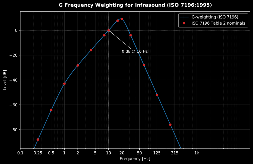
3. Infrasound: G-weighting (ISO 7196)

The G frequency weighting (ISO 7196:1995) rates infrasound the way A-weighting rates audible noise. It is defined by a pole-zero configuration with 0 dB gain at 10 Hz, rises at 12 dB/octave from 1 Hz to 20 Hz (matching the steep growth of perception in that band) and falls off at 24 dB/octave outside it. Use it for sources with significant energy below 20 Hz (wind turbines, HVAC, blasting):

import numpy as np
from phonometry import metrology

# recording: a calibrated microphone capture (Pa) — recorded through your measurement chain. Synthesized here so the guide runs standalone.
fs = 48000
recording = 0.2 * np.sin(2 * np.pi * 1000 * np.arange(fs) / fs)

g_weighted = metrology.weighting_filter(recording, fs, curve='G')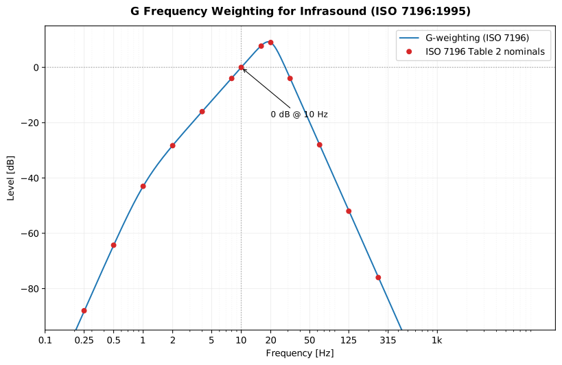

Show the code for this figure

import matplotlib.pyplot as plt
import numpy as np
from phonometry import metrology

# Measure the G response: weight a centered unit impulse and take its
# spectrum. A long buffer gives the resolution the infrasound range
# needs (20 s -> 0.05 Hz).
fs = 4000
impulse = np.zeros(20 * fs)
impulse[impulse.size // 2] = 1.0
freqs = np.fft.rfftfreq(impulse.size, 1 / fs)
spectrum = np.fft.rfft(metrology.weighting_filter(impulse, fs, curve="G"))

fig, ax = plt.subplots(figsize=(9, 5))
ax.semilogx(freqs[1:],
            20 * np.log10(np.abs(spectrum[1:]) + np.finfo(float).eps))
ax.plot(10, 0, "o", color="tab:red", label="0 dB at 10 Hz")
ax.set(xlim=(0.1, 1000), ylim=(-90, 15),
       xlabel="Frequency [Hz]", ylabel="G-weighting response [dB]")
ax.grid(True, which="both", alpha=0.3)
ax.legend()
plt.show()

The implementation follows the ISO 7196 Table 1 pole/zero values exactly and is verified in CI against every Table 2 nominal response value (0.25 Hz to 315 Hz). WeightingFilter(fs, "G") supports the same multichannel and stateful block processing as A/C. Levels measured with the G curve are reported as L_pG (or L_Geq for the equivalent level over time).

4. Historical and special-purpose curves: B, D and AU

Three more curves complete the family. All three share the machinery of the IEC 61672-1 curves (0 dB at 1 kHz, high_accuracy oversampling, multichannel and stateful block processing).

B (ANSI S1.4-1983, historical)

The middle curve of the original A/B/C level-switching scheme, drawn from the ~70-phon equal-loudness contour. Analytically it is the C weighting with one more zero at the origin and one extra real pole at $f_5=158.49\text{Hz}$ (Appendix C of ANSI S1.4-1983), so it discards less bass than A and more than C. It was dropped when IEC 61672-1 replaced the older sound-level-meter standards; use it only to reproduce historical data and measurements taken under older national codes (some legacy automotive test procedures reported dB(B)). The implementation follows the ANSI S1.4-1983 Appendix C constants and is pinned in CI against the Table IV response values, within the strictest Table V mask (Type 0).

D (IEC 537, withdrawn: aircraft noise)

The D weighting approximated the perceived noisiness contours used by the perceived-noise-level (PNL) rating, so a plain sound level meter could estimate aircraft noise: the +11.5 dB hump around 3.15 kHz is where jet turbomachinery whine annoys most (it is deliberately not an equal-loudness feature). NASA’s aircraft-noise handbook gives the classic rule of thumb $L_{PN}\approx L_D+7\text{dB}$. IEC 537 was withdrawn and current certification practice reports EPNL from one-third-octave analysis or plain A-weighted levels, so D is provided for historical data and comparisons. With the standard unavailable, the implementation uses the widely published IEC 537 rational transfer function and is cross-checked against two independent implementations (SQAT’s zeros/poles and librosa’s closed form, which agree within 0.002 dB) and pinned in CI against the IEC 537 table republished in NASA CR-3406.

import numpy as np
from phonometry import metrology

# A 3.15 kHz whine sits right on the D-weighting hump: D rates it
# 10 dB *louder* than A does.
fs = 96000
t = np.arange(fs) / fs
whine = 0.1 * np.sin(2 * np.pi * 3150 * t)

ld = metrology.leq(metrology.weighting_filter(whine, fs, curve="D"))
la = metrology.leq(metrology.weighting_filter(whine, fs, curve="A"))
print(f"LD = {ld:.1f} dB   LA = {la:.1f} dB")
# LD = 82.5 dB   LA = 72.2 dB

AU (IEC 61012, current: audible sound in the presence of ultrasound)

The only one of the three still in force. AU is the A weighting cascaded with the U low-pass filter of IEC 61012:1990 (six poles, Table 2): flat relative to A up to 10 kHz, then a steep cutoff (-13 dB at 16 kHz, -61.8 dB at 40 kHz for U alone). Use it when strong ultrasonic components (ultrasonic cleaners and welders, rodent repellers, some public-space deterrents) would otherwise leak into an A-weighted reading through the meter’s imperfect high-frequency roll-off and overstate the audible exposure:

import numpy as np
from phonometry import metrology

# 1 kHz tone (audible) buried under a strong 25 kHz ultrasonic component.
fs = 96000
t = np.arange(fs) / fs
audible = 0.1 * np.sin(2 * np.pi * 1000 * t)
x = audible + 1.0 * np.sin(2 * np.pi * 25000 * t)

la = metrology.leq(metrology.weighting_filter(x, fs, curve="A"))
lau = metrology.leq(metrology.weighting_filter(x, fs, curve="AU"))
la_ref = metrology.leq(metrology.weighting_filter(audible, fs, curve="A"))
print(f"LA = {la:.1f} dB   LAU = {lau:.1f} dB   audible alone = {la_ref:.1f} dB")
# LA = 78.6 dB   LAU = 71.0 dB   audible alone = 71.0 dB
# The ultrasound inflates LA by 7.6 dB; AU recovers the audible level.

Ultrasound only reaches a digital filter when the sample rate captures it, so measure at 96 kHz or more (at 48 kHz there is nothing above 24 kHz to reject); the AU design internally oversamples toward 288 kHz to keep the steep U roll-off accurate. Levels are reported as L_AU. The implementation follows the Table 2 pole locations exactly (they reproduce every Table 1 nominal value within 0.05 dB) and is verified in CI against the Table 1 tolerances up to 40 kHz.

5. weighting_filter() / WeightingFilter parameters

Parameter	Type	Units	Range / default	Notes
x	1D or 2D array	any	non-empty	2D is [channels, samples]
fs	int	Hz	> 0
curve	str	—	'A' (default), 'B', 'C', 'D', 'G', 'AU', 'Z'	'G' per ISO 7196 (infrasound); 'B'/'D' historical (§4); 'AU' per IEC 61012 (§4); 'Z' is a bypass
high_accuracy	bool	—	default True (function); class default None resolves to not stateful	Internal oversampling keeps A/C in class 1 up to 16 kHz; details in §7
stateful	bool (class only)	—	default False	Carries filter state across blocks (streaming)
steady_ic	bool (class only)	—	default False	Steady-state initial conditions (no onset transient)

6. Reusable filter object

If you weight many signals with the same parameters, design the filter once:

import numpy as np
from phonometry import metrology

# recording: a calibrated microphone capture (Pa) — recorded through your measurement chain. Synthesized here so the guide runs standalone.
fs = 48000
recording = 0.2 * np.sin(2 * np.pi * 1000 * np.arange(fs) / fs)

wf = metrology.WeightingFilter(fs, "A")
signals = [recording]                # your batch of recordings
for recording in signals:
    weighted = wf.filter(recording)

7. High-frequency accuracy (high_accuracy)

A plain bilinear-transform design compresses the response near Nyquist: at fs = 48 kHz the A-curve error at 12.5 kHz reaches −2.7 dB, outside the IEC 61672-1 class 1 tolerance (+2.0/−2.5 dB).

By default (high_accuracy=True), phonometry designs and runs the weighting filter at an internally oversampled rate (up to 8×, reaching ≥ 144 kHz at common audio rates; a 96 kHz input runs ×2) and decimates back, keeping the response within class 1 tolerances up to 16 kHz (error ≈ −0.5 dB at 12.5 kHz for fs = 48 kHz).

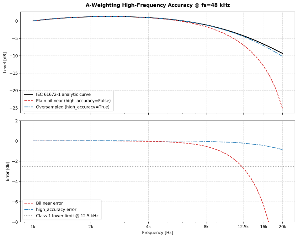
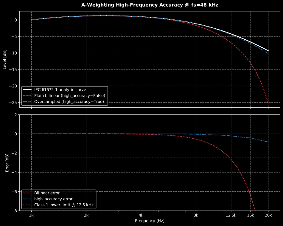
The plain bilinear design (red) crosses the class 1 tolerance near 12.5 kHz; the oversampled design (blue) stays close to the analytic curve.

Show the code for this figure

import matplotlib.pyplot as plt
import numpy as np
from phonometry import metrology

# Measured response of both designs at fs = 48 kHz: weight a centered
# unit impulse and take its spectrum...
fs = 48000
impulse = np.zeros(fs)
impulse[fs // 2] = 1.0
freqs = np.fft.rfftfreq(fs, 1 / fs)[1:]

# ...versus the analytic IEC 61672-1 A-curve built from the four corner
# frequencies of section 1, normalized to 0 dB at 1 kHz.
f1, f2, f3, f4 = 20.599, 107.653, 737.862, 12194.217
gain = (f4**2 * freqs**4) / ((freqs**2 + f1**2)
        * np.sqrt((freqs**2 + f2**2) * (freqs**2 + f3**2))
        * (freqs**2 + f4**2))
analytic = 20 * np.log10(gain / gain[np.argmin(np.abs(freqs - 1000))])

fig, ax = plt.subplots(figsize=(9, 5))
ax.semilogx(freqs, analytic, "k--", label="Analytic (IEC 61672-1)")
for high_accuracy, label in ((False, "Plain bilinear"),
                             (True, "Oversampled (default)")):
    weighted = metrology.weighting_filter(impulse, fs, curve="A",
                                high_accuracy=high_accuracy)
    response = 20 * np.log10(np.abs(np.fft.rfft(weighted))
                             + np.finfo(float).eps)[1:]
    ax.semilogx(freqs, response, label=label)
ax.set(xlim=(1000, 20000), ylim=(-12, 3),
       xlabel="Frequency [Hz]", ylabel="A-weighting response [dB]")
ax.grid(True, which="both", alpha=0.3)
ax.legend()
plt.show()

• high_accuracy=False restores the legacy plain-bilinear behavior.
• For 'G' the flag is silently ignored: its 0.25–315 Hz range is already exact with the plain design.
• Stateful (block) processing always uses the legacy design: the internal FIR resampling is incompatible with block continuity. Passing high_accuracy=True together with stateful=True raises a ValueError.

import numpy as np
from phonometry import metrology

# recording: a calibrated microphone capture (Pa) — recorded through your measurement chain. Synthesized here so the guide runs standalone.
fs = 48000
recording = 0.2 * np.sin(2 * np.pi * 1000 * np.arange(fs) / fs)

# Explicit legacy behavior
y = metrology.weighting_filter(recording, fs, curve="A", high_accuracy=False)

# Stateful block processing (legacy design, state carried between blocks)
wf = metrology.WeightingFilter(fs, "A", stateful=True)
blocks = [recording]                 # your sequence of recording blocks
for block in blocks:
    weighted = wf.filter(block)

See Block Processing for the streaming workflow and Theory for the analytic curve definitions.

8. Verifying against the tolerance tables (IEC 61672-1, ANSI S1.4, IEC 61012)

verify_weighting_class checks a weighting filter against the acceptance limits of IEC 61672-1:2013 (Table 3). It evaluates the filter’s relative response at the exact base-10 frequency behind each nominal label below Nyquist (Table 3’s design goals are computed at $f=1000\cdot 10^{n/10}$, e.g. 15 848.9 Hz for “16 kHz”; IEC 61672-3 tests at the same frequencies), subtracts the design-goal weighting, and reports the performance class per frequency with its margin in dB. A dense logarithmic sweep additionally enforces subclause 5.5.7 between the nominal frequencies (the deviation from the analytic Annex E goal must stay within the larger of the two adjacent limits, so a resonance or notch between nominals cannot pass), and when Table 3 rows with finite lower limits fall beyond Nyquist the verdict is flagged range_limited (it then attests the checked frequencies only, not full 10 Hz-20 kHz conformance):

from phonometry import metrology

result = metrology.verify_weighting_class(metrology.WeightingFilter(48000, "A"))
print(result["overall_class"])          # 1
print(result["range_limited"])          # False
print(result["between_nominals"])       # {'worst_freq': ..., 'margin_class1_db': ...}
print(result["bands"][20])
# {'freq': 1000.0, 'class': 1, 'deviation_db': 0.0, 'margin_class1_db': 0.7, 'margin_class2_db': 1.0}

The Table 3 acceptance mask itself is public too: weighting_class_limits(1) returns the 34 nominal frequencies with the lower/upper deviation limits (a lower limit of -inf means only the upper limit applies). The limits qualify the deviation from the design goal, so they are the same for A, C and Z.

The same verifier covers the section 4 curves that have published tolerance tables. For B it uses ANSI S1.4-1983 (Table IV design goals, Table V limits) and the “class” verdicts read as the standard’s instrument Types 1 and 2. For AU it uses IEC 61012:1990 Table 1 (nominal A + nominal U with the separate-unit tolerances, zero at the 1 kHz reference); IEC 61012 publishes a single tolerance set, so both margin slots agree and the verdict is simply complies (1) or not (None) — note that checking the rows above 20 kHz needs fs ≥ 96 kHz (below that they are dropped and the verdict is range_limited). G and D are rejected: ISO 7196 defines one ±1 dB tolerance with no class structure, and the withdrawn IEC 537 left no tolerance table behind (both curves are pinned numerically in the CI conformance report instead).

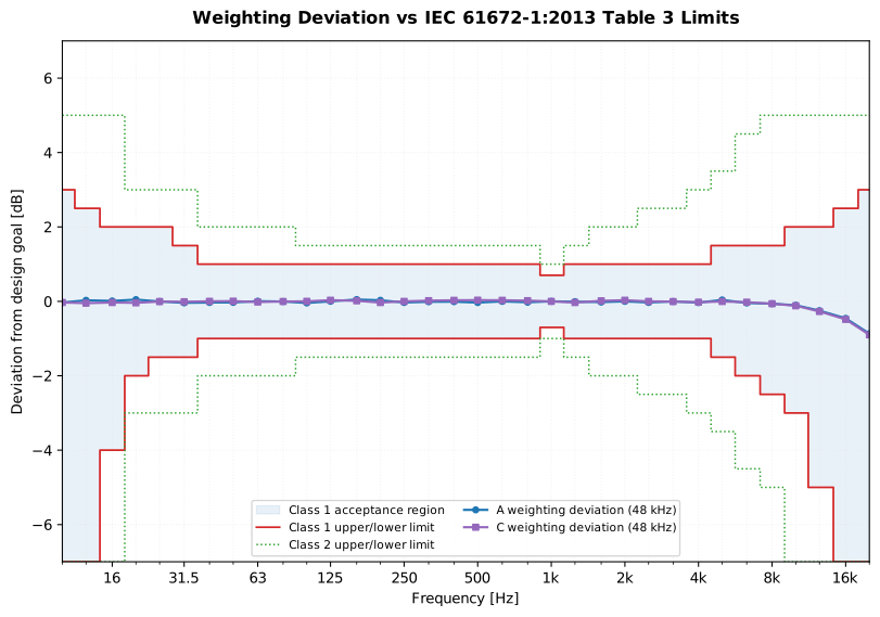
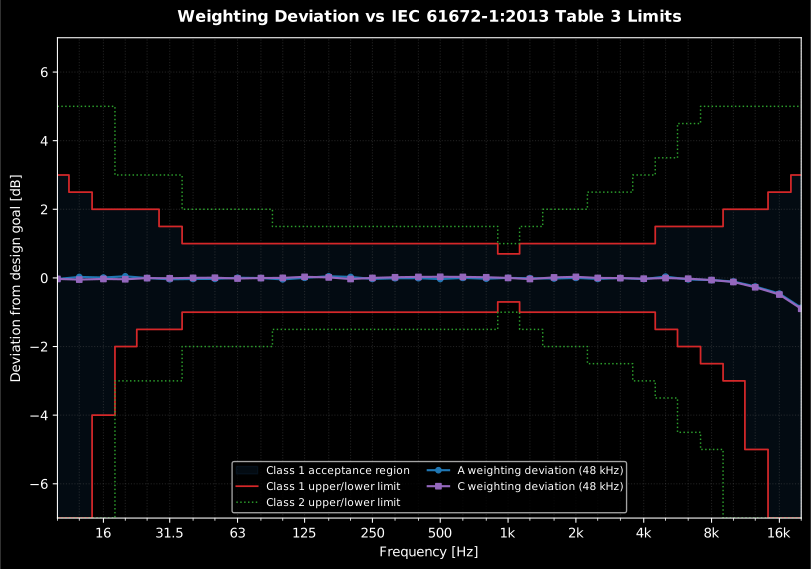
The oversampled A and C designs (blue, purple) stay near zero deviation, well inside the class 1 corridor (shaded); the wider class 2 limits are dotted. The corridor widens at the band extremes where only a one-sided limit applies.

Show the code for this figure

import matplotlib.pyplot as plt
import numpy as np
from phonometry import metrology

freqs, lower1, upper1 = metrology.weighting_class_limits(1)
_, lower2, upper2 = metrology.weighting_class_limits(2)
lo1, lo2 = np.clip(lower1, -7, 7), np.clip(lower2, -7, 7)

fig, ax = plt.subplots(figsize=(10, 6.5))
ax.fill_between(freqs, lo1, upper1, step="mid", alpha=0.10,
                label="Class 1 acceptance region")
ax.plot(freqs, upper1, drawstyle="steps-mid", label="Class 1 upper/lower limit")
ax.plot(freqs, lo1, drawstyle="steps-mid", color="C1")
ax.plot(freqs, upper2, ":", drawstyle="steps-mid", label="Class 2 upper/lower limit")
ax.plot(freqs, lo2, ":", drawstyle="steps-mid", color="C2")

for curve, marker in (("A", "o"), ("C", "s")):
    bands = metrology.verify_weighting_class(metrology.WeightingFilter(48000, curve))["bands"]
    f = [b["freq"] for b in bands]
    dev = [b["deviation_db"] for b in bands]
    ax.plot(f, dev, marker=marker, label=f"{curve} weighting deviation (48 kHz)")

ax.set(xscale="log", xlim=(10, 20000), ylim=(-7, 7),
       xlabel="Frequency [Hz]", ylabel="Deviation from design goal [dB]")
ax.legend(fontsize=8, ncol=2)
plt.show()

What this guide covers

Covered. IEC 61672-1:2013 for the A, C and Z curves: the Annex E analytic definition from four corner frequencies, the high_accuracy design that keeps class 1 tolerances up to 16 kHz, and the Table 3 class 1/class 2 acceptance limits checked by verify_weighting_class. ISO 7196:1995 for the G curve (Table 1 pole/zero values, verified against every Table 2 nominal response). ANSI S1.4-1983 for the historical B curve (Appendix C definition, Table IV design goals, Table V tolerance limits). IEC 61012:1990 for AU (the U low-pass of Table 2 cascaded with A, verified against Table 1). IEC 537:1976 for the withdrawn aircraft-noise D curve, implemented from its published transfer function and cross-checked against two independent implementations.

Not covered. verify_weighting_class does not produce a class verdict for G or D: ISO 7196 defines a single ±1 dB tolerance with no class structure, and the withdrawn IEC 537 left no tolerance table behind. Both curves are pinned numerically against their published tables in the CI conformance report instead, not through this public verifier. B and D are provided for historical data and older national codes only; neither is current practice (IEC 61672-1 replaced B, and aircraft-noise certification now reports EPNL or plain A-weighted levels instead of D).

See also

• API reference: metrology.parametric_filters and metrology.compliance.

Quick answers

When should I use C-weighting instead of A-weighting?

Use C-weighting for peak sound pressure and high-level noise, and use the difference $L_{Ceq}-L_{Aeq}$ as a low-frequency indicator: below about 10 dB the A-weighted level rates the spectrum fairly, while around 15 to 20 dB or more the energy is concentrated at low frequencies and the A-weighted level understates the problem. The HML method of ISO 4869-2 keys on exactly this C minus A difference for hearing-protector selection.

Which weighting should I use for infrasound below 20 Hz?

Use the G frequency weighting of ISO 7196:1995, which rates infrasound the way A-weighting rates audible noise. It has 0 dB gain at 10 Hz, rises at 12 dB/octave from 1 Hz to 20 Hz and falls off at 24 dB/octave outside that band. Apply it to sources such as wind turbines, HVAC and blasting, and report levels as $L_{pG}$ (or $L_{Geq}$ for the equivalent level over time).

Is A-weighting accurate near 16 kHz at a 48 kHz sample rate?

Not with a plain bilinear design: at fs = 48 kHz the A-curve error reaches −2.7 dB at 12.5 kHz, outside the IEC 61672-1 class 1 tolerance (+2.0/−2.5 dB). The default high_accuracy=True oversamples internally (up to 8×, reaching 144 kHz or more at common audio rates) and keeps the response within class 1 tolerances up to 16 kHz, with an error of about −0.5 dB at 12.5 kHz.

References

• American National Standards Institute. (1983). Specification for Sound Level Meters (ANSI S1.4-1983). The historical B weighting: Appendix C analytic definition (Formula C2), Table IV design goals and Table V tolerance limits checked by verify_weighting_class in section 8.
• Bennett, R. L., & Pearsons, K. S. (1981). Handbook of Aircraft Noise Metrics (NASA CR-3406). NASA. Republishes the IEC 537 D-weighting table (Table SLD-I) used to pin the D response in CI.
• Fletcher, H., & Munson, W. A. (1933). Loudness, its definition, measurement and calculation. The Journal of the Acoustical Society of America, 5(2), 82-108. https://doi.org/10.1121/1.1915637The original equal-loudness measurements whose 40-phon contour the A-curve inverts (section 1).
• International Electrotechnical Commission. (1976). Frequency weighting for the measurement of aircraft noise (D-weighting) (IEC 537:1976 (withdrawn)). The D weighting, implemented from its published rational transfer function and cross-checked against two independent implementations and the tabulated curve republished in NASA CR-3406 (Table SLD-I).
• International Electrotechnical Commission. (1990). Filters for the measurement of audible sound in the presence of ultrasound (IEC 61012:1990). The AU weighting: U-weighting pole locations (Table 2), nominal responses and tolerances (Table 1) and the combined AU definition of subclause 2.2.
• International Electrotechnical Commission. (2013). Electroacoustics — Sound level meters — Part 1: Specifications (IEC 61672-1:2013). The normative A, C and Z frequency-weighting curves (the Annex E analytic definition from four corner frequencies, normalized to 0 dB at 1 kHz), the class 1 tolerances the high_accuracy design keeps up to 16 kHz, and the Table 3 class 1/class 2 acceptance limits checked by verify_weighting_class in section 8.
• International Organization for Standardization. (1995). Acoustics — Frequency-weighting characteristic for infrasound measurements (ISO 7196:1995). The G-weighting pole/zero definition (Table 1), verified against every Table 2 nominal response value (0.25 Hz to 315 Hz).
• International Organization for Standardization. (2023). Acoustics — Normal equal-loudness-level contours (ISO 226:2023). The modern successors of the Fletcher-Munson curves, drawn in the diagram of section 1.