Hearing threshold (age and reference zero)

Two standards describe where the hearing threshold sits. ISO 7029:2017 gives the statistical distribution of the hearing threshold with age for an otologically normal population: the slow, high-frequency-first loss known as presbycusis. ISO 389-7:2005 fixes the reference threshold of hearing, the audiometric zero (0 dB HL) expressed as a sound pressure level under free-field and diffuse-field listening. Both are defined over the audiometric frequencies from 125 Hz to 8000 Hz.

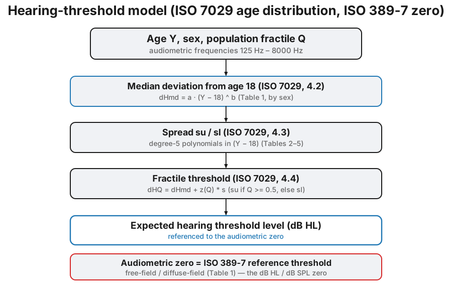
1. Age-related threshold (ISO 7029)

For a person older than 18, the median hearing threshold deviation from the value at age 18 grows as a power law of age (ISO 7029 clause 4.2, Table 1):

$$\Delta H_{md}=a(Y-18{)}^b,$$

with coefficients $a$, $b$ per frequency and sex. The spread around the median is modelled by two half-Gaussians whose standard deviations $s_u$ (worse than the median) and $s_l$ (better) are fifth-degree polynomials in $(Y-18)$ (clause 4.3, Tables 2–5). Any population fractile $Q$ follows from the standard-normal quantile $z(Q)$ (clause 4.4): $\Delta H_Q=\Delta H_{md}+z(Q)s$, using $s_u$ when $z\ge 0$ and $s_l$ otherwise.

from phonometry import hearing

# Median threshold shift of a 65-year-old man, all audiometric frequencies.
result = hearing.age_threshold(65, "male", fractile=0.5)
print(result.median.round(1))     # [ 6.6  7.6  8.  9.  10.4 13.4 16.3 21.6 26.2 33.7 39.5]
print(result.median[8].round(1))  # 26.2 dB at 4000 Hz

# The worst-hearing decile (90th percentile) at 4000 Hz:
print(hearing.age_threshold(65, "male", fractile=0.9).threshold[8].round(1))  # 50.3

result.plot()   # the median with the 10-90 % fractile band (needs matplotlib)

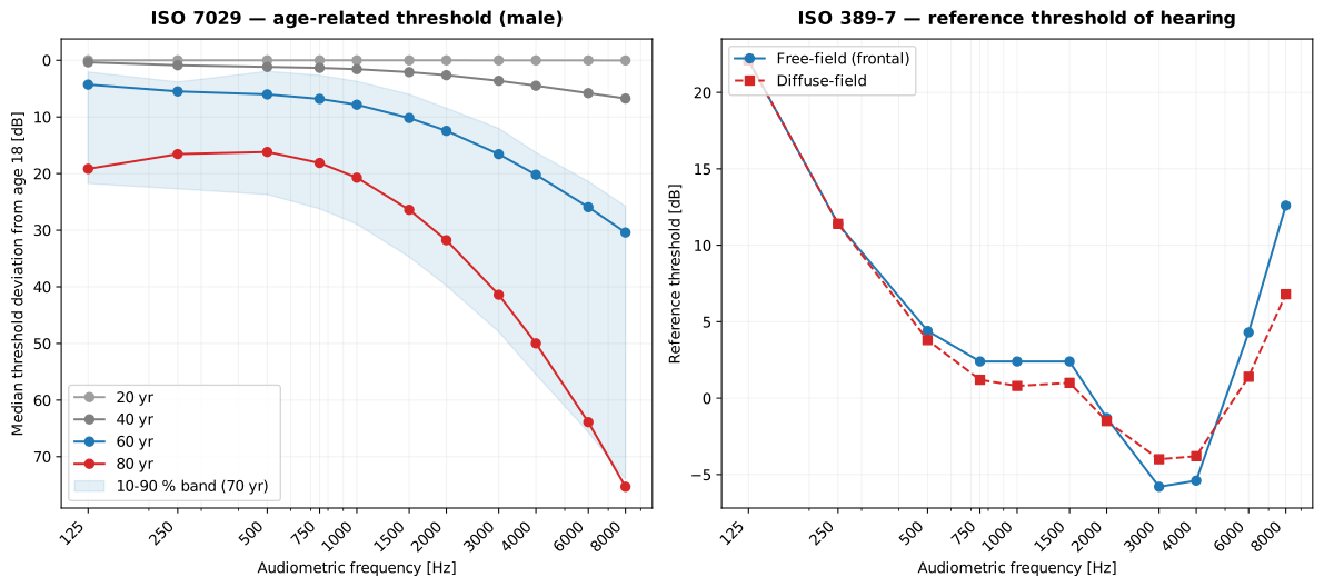
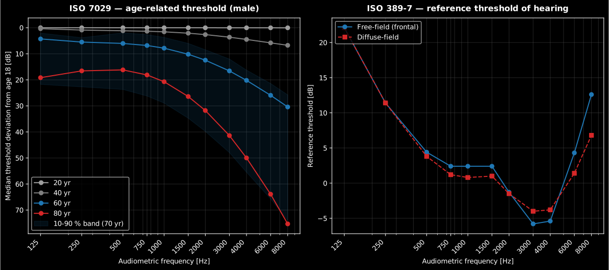
The loss is largest at the high frequencies and grows with age: the classic downward-sloping presbycusis audiogram. Men and women follow different coefficients (the sex argument), and a subset of the audiometric frequencies can be requested with frequencies=.

Who counts as “otologically normal”. The ISO 7029 population is not the general population: it is people screened to be in a normal state of health, free from signs or symptoms of ear disease and wax obstruction, and (the demanding part) with no history of undue noise exposure, ototoxic drugs or familial hearing loss. The model therefore isolates pure ageing: it is the baseline that other standards subtract from. A real, unscreened workforce tends to have higher thresholds on average (not necessarily at every age or frequency), which is why ISO 1999 supplies an unscreened population as an alternate reference (its “database B”) for studies whose goal is comparison with an actual population rather than isolating the noise effect.

Reading the percentiles. A fractile is a population statement, not a prediction for a person: fractile=0.9 returns the threshold that 90 % of otologically normal people of that age and sex are better than (only the worst-hearing tenth exceeds it), and fractile=0.5 the median: half above, half below. The spread is deliberately asymmetric (two half-Gaussians, $s_u>s_l$): ageing drags a minority far down while the better-hearing half stays bunched near the median, so the far percentiles on the bad side move much faster with age than the good side ever improves. An individual audiogram can sit anywhere in that fan; the model tells you how surprising it is, not what it should be.

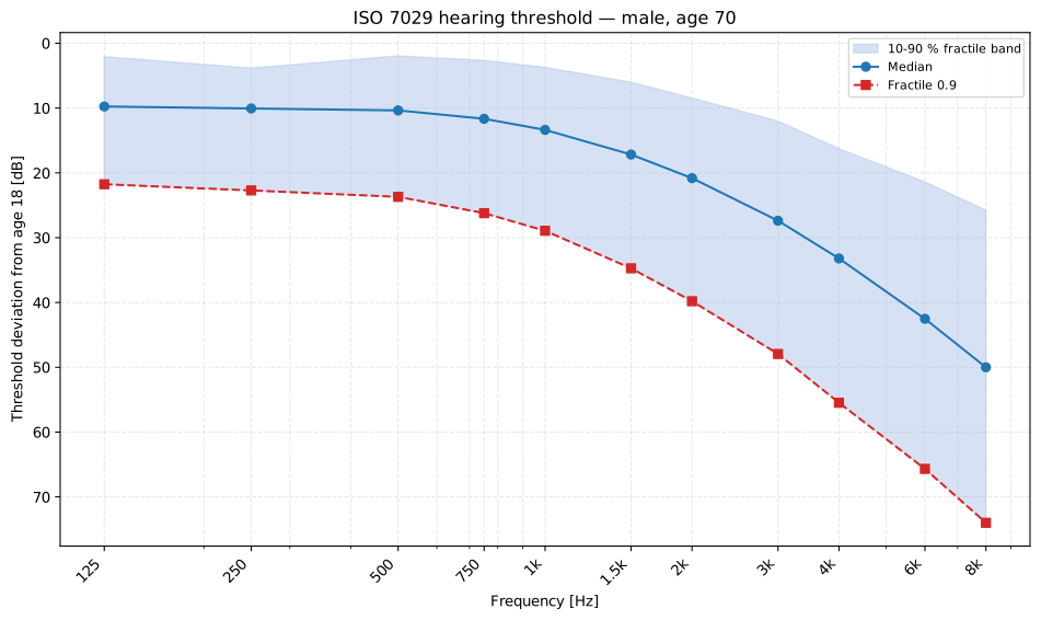
AgeThresholdResult.plot() draws that fan directly: the median, the requested fractile and the 10 % to 90 % band between them, on an audiogram axis.

Show the code for this figure

import matplotlib.pyplot as plt
from phonometry import hearing

# A 70-year-old man, worst-hearing decile: the median presbycusis slope with
# the population spread around it.
res = hearing.age_threshold(70, "male", fractile=0.9)
print(res.median.round(1))
print(res.threshold.round(1))     # the 90 % fractile

# One line: the median, the fractile and the 10-90 % band.
res.plot()
plt.show()

The band is the whole point of the model. At 500 Hz the fractiles of a 70-year-old span a handful of decibels, so an individual audiogram there is informative; at 8 kHz they span tens of decibels, so a single measured value says little about whether that ear is unusual. Any statement of the form “this person has lost more hearing than their age explains” is a statement about where they sit in this fan, and it needs the fractile, not the median.

Where the age component goes next. ISO 7029 is not only an audiology reference: it is the age input of the noise-induced-hearing-loss model. ISO 1999:2013 calls it database A and its clause 6.1 Formula (1) combines the age threshold H with the noise-induced shift N into the threshold a real audiogram would show, H' = H + N - HN/120, at the same fractile. In practice that means the two guides chain: pick the population and fractile here, add the exposure there, and compare the result, never the noise component alone, against a measured audiogram. The noise-induced hearing loss guide picks the chain up at that point.

2. Reference threshold of hearing (ISO 389-7)

The audiometric zero is not a fixed sound pressure level: it depends on how the sound reaches the listener. ISO 389-7:2005 Table 1 gives the reference threshold for free-field (frontal incidence) and diffuse-field listening.

from phonometry import hearing

print(hearing.reference_threshold("free-field"))
# [22.1 11.4  4.4  2.4  2.4  2.4 -1.3 -5.8 -5.4  4.3 12.6]
print(hearing.reference_threshold("diffuse-field")[4])   # 0.8 dB at 1000 Hz

The two fields agree at low frequencies and diverge above about 1 kHz, where the ear-canal resonance and head diffraction make the frontal free field the more sensitive condition (a lower threshold) around 3–4 kHz.

Show the code for this figure

import matplotlib.pyplot as plt
from phonometry import hearing
from phonometry.hearing import AUDIOMETRIC_FREQUENCIES as f

# One line for the age distribution:
hearing.age_threshold(70, "male", 0.5).plot()
plt.show()

# By hand, both panels:
fig, (ax1, ax2) = plt.subplots(1, 2, figsize=(12, 5))
for age in (20, 40, 60, 80):
    r = hearing.age_threshold(age, "male", 0.5)
    ax1.plot(f, r.median, "o-", label=f"{age} yr")
ax1.set_xscale("log"); ax1.invert_yaxis(); ax1.legend()

ax2.plot(f, hearing.reference_threshold("free-field"), "o-", label="Free-field")
ax2.plot(f, hearing.reference_threshold("diffuse-field"), "s--", label="Diffuse-field")
ax2.set_xscale("log"); ax2.legend()
plt.show()

The AgeThresholdResult carries the median, the spread_upper and spread_lower, and the threshold at the requested fractile, and its .plot() draws the median with the 10–90 % band. The noise-induced permanent threshold shift of ISO 1999, which adds a noise component on top of this age component, is the subject of the noise-induced hearing loss guide.

What this guide covers

Covered. ISO 7029:2017’s age model: the median power-law deviation from age 18 (clause 4.2, Table 1), the asymmetric half-Gaussian spreads $s_u$ and $s_l$ (clause 4.3, Tables 2–5), and the population-fractile calculation of clause 4.4, all implemented by age_threshold(age, sex, fractile). ISO 389-7:2005 Table 1’s free-field and diffuse-field reference threshold of hearing, returned by reference_threshold(field).

Not covered. ISO 1999:2013 clause 6.1 Formula (1) combines this age threshold with a noise-induced shift into a real audiogram. That noise component is not implemented here: it is the subject of the noise-induced hearing loss guide. Of ISO 389-7:2005, this module implements only the Table 1 reference values; the rest of the standard, including how those values were established, is not implemented.

See also

• Noise-induced hearing loss: the ISO 1999 model that adds the noise component on top of this age component.
• Speech Intelligibility Index: a raised threshold as an input, and what it costs in speech audibility.
• Loudness: the ISO 226:2023 threshold of hearing, the free-field pure-tone counterpart of the audiometric zero of section 2.
• Occupational noise exposure: the ISO 9612 daily exposure level that drives the noise component.
• API reference: hearing.threshold.

References

• International Organization for Standardization. (2005). Acoustics — Reference zero for the calibration of audiometric equipment — Part 7: Reference threshold of hearing under free-field and diffuse-field listening conditions (ISO 389-7:2005). The audiometric zero of section 2 (Table 1), implemented here through its European adoption EN ISO 389-7:2006.
• International Organization for Standardization. (2017). Acoustics — Statistical distribution of hearing thresholds related to age and gender (ISO 7029:2017). The age model of section 1: the median power law (clause 4.2, Table 1), the asymmetric spread around the median (clause 4.3, Tables 2–5) and the fractile machinery and its application (clause 4.4).