Prominent Discrete Tones (ECMA-418-1)

By José M. Requena Plens · Published Jul 10, 2026, updated Jul 26, 2026

Tonal components in machinery noise are far more annoying than their level suggests. ECMA-418-1:2024 (referenced by ECMA-74 Annex D) gives two FFT-based methods to decide whether a discrete tone is prominent: tone_to_noise_ratio() compares the tone level with the masking noise in its critical band (clause 11), and prominence_ratio() compares the critical band centred on the tone with the two contiguous bands (clause 12). Both return a structured verdict against the frequency-dependent prominence criteria.

1. Tone-to-noise ratio and prominence ratio

import numpy as np
from phonometry import psychoacoustics

fs = 48000
rng = np.random.default_rng(0)
t = np.arange(fs) / fs
x = np.sin(2 * np.pi * 1000 * t) + 0.05 * rng.standard_normal(fs)  # 1 kHz tone in noise
tnr = psychoacoustics.tone_to_noise_ratio(x, fs)            # highest peak, or tone_freq=...
pr = psychoacoustics.prominence_ratio(x, fs, tone_freq=1000.0)
print(tnr.ratio_db, tnr.criterion_db, tnr.prominent)

tnr.plot()   # the tone against its prominence criterion (needs matplotlib)

The methods hinge on the critical band, the ear’s analysis bandwidth, $Δ f_{c} = 25 + 75 [1 + 1.4 (f /1000)^{2}]^{0.69}$ Hz (162 Hz at 1 kHz): a tone is masked only by the noise inside its critical band, so both methods focus on that band rather than the whole spectrum, but they use it differently. The tone-to-noise ratio works within the band, separating its spectral lines into tone and noise and subtracting their levels (clause 11, Formulae 9–11); the prominence ratio instead compares the whole band centred on the tone with the mean of its two contiguous critical bands (clause 12, Formula 23):

TNR = L_{t} - L_{n}, PR = 10 l g \frac{W _{M}}{\frac{1}{2} ( W _{L} + W _{U} )} dB,

where $L_{t}$ is the tone level (the energy sum of the tonal lines above the band-edge baseline, Formula 9), $L_{n}$ the level of the masking noise that remains in the critical band, rescaled to the full critical bandwidth (Formulae 10–11), and $W_{M}$ , $W_{L}$ , $W_{U}$ the powers in the middle, lower and upper critical bands (below $f_{t} = 171.4$ Hz the truncated lower band is rescaled to a 100 Hz bandwidth, Formula 24).

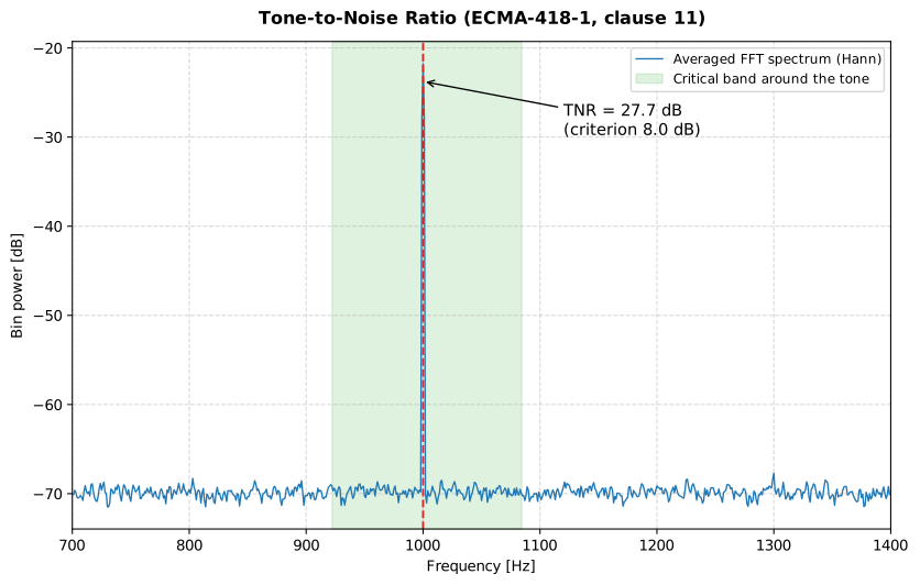
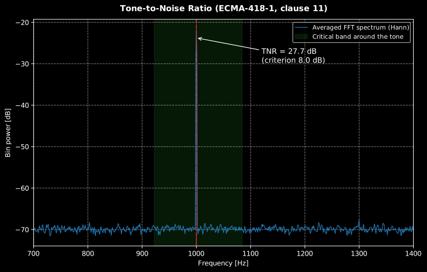
Averaged spectrum of a tone in noise with the critical band shaded and the tone-to-noise ratio annotated against its prominence criterion

Show the code for this figure

import numpy as np
import matplotlib.pyplot as plt
from scipy.signal import welch
from phonometry import psychoacoustics

fs = 48000
rng = np.random.default_rng(21)
t = np.arange(30 * fs) / fs
x = (np.sqrt(2) * 0.1 * np.sin(2 * np.pi * 1000 * t)
     + 0.05 * rng.standard_normal(t.size))
res = psychoacoustics.tone_to_noise_ratio(x, fs)

# Averaged 1 Hz Hann spectrum (the clause 11.1 front end) and the
# critical band about the detected tone (edges approximated as +/- dfc/2):
f, p = welch(x, fs, window="hann", nperseg=fs, scaling="spectrum")
dfc = 25 + 75 * (1 + 1.4 * (res.frequency / 1000) ** 2) ** 0.69
sel = (f > 700) & (f < 1400)
plt.plot(f[sel], 10 * np.log10(p[sel]))
plt.axvspan(res.frequency - dfc / 2, res.frequency + dfc / 2, alpha=0.15)
plt.title(f"TNR = {res.ratio_db:.1f} dB (criterion {res.criterion_db:.1f} dB)")
plt.xlabel("Frequency [Hz]"); plt.ylabel("Bin power [dB]")
plt.show()

A TNR at or above $8 + 8.33 lo g_{10} (1000/ f_{t})$ dB below 1 kHz (a flat 8 dB for $f_{t} \geq 1$ kHz) classifies the tone as prominent; the PR criterion is $9 + 10 lo g_{10} (1000/ f_{t})$ dB below 1 kHz and 9 dB from there up, likewise applied with $\geq$ . Low frequencies get higher thresholds because wider relative bands mask more.

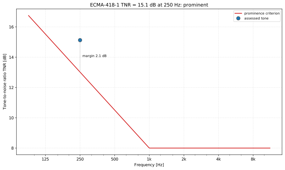
ToneAssessment.plot() puts the verdict in its context: it draws the criterion of the producing method over the whole 89.1 Hz to 11.2 kHz range of interest and marks the assessed tone at its own frequency, so the margin that decides the verdict is visible rather than implied.

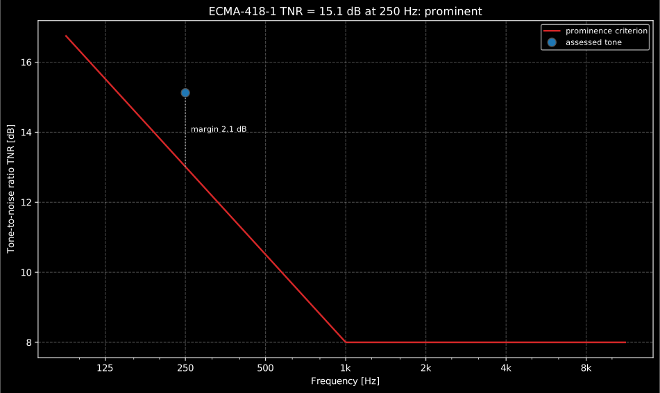
Tone-to-noise ratio of a 250 Hz fan tone plotted against the ECMA-418-1 prominence criterion: the criterion falls from about 17 dB at 89 Hz to a flat 8 dB above 1 kHz, and the assessed tone sits at 15.1 dB, 2.1 dB above the 13.0 dB criterion at 250 Hz, so it is prominent

Show the code for this figure

import numpy as np
import matplotlib.pyplot as plt
from phonometry import psychoacoustics

# A 250 Hz fan tone recorded in broadband machinery noise, 10 s at 48 kHz.
fs = 48000
rng = np.random.default_rng(4)
t = np.arange(10 * fs) / fs
x = (np.sqrt(2) * 0.011 * np.sin(2 * np.pi * 250.0 * t)
     + 0.03 * rng.standard_normal(t.size))
res = psychoacoustics.tone_to_noise_ratio(x, fs)
print(round(res.ratio_db, 1), round(res.criterion_db, 1), res.prominent)
# 15.1 13.0 True

# One line: the tone against the criterion curve of its own method.
res.plot()
plt.show()

# By hand, mirroring what ToneAssessment.plot() draws:
f = np.logspace(np.log10(89.1), np.log10(11200.0), 400)
criterion = np.where(f < 1000.0, 8.0 + 8.33 * np.log10(1000.0 / f), 8.0)
fig, ax = plt.subplots()
ax.semilogx(f, criterion, color="#d62728", label="prominence criterion")
ax.plot([res.frequency], [res.ratio_db], "o", label="assessed tone")
ax.plot([res.frequency] * 2, [res.criterion_db, res.ratio_db], ":", color="0.6")
ax.set_xlabel("Frequency [Hz]")
ax.set_ylabel("Tone-to-noise ratio TNR [dB]")
ax.legend()
plt.show()

When the two ratios disagree. Near the criteria the verdicts can differ, because each ratio is fragile in a different situation. TNR has to split the critical band into tonal and noise lines first, so it degrades when that separation is ambiguous: a tone riding a steep noise slope, or closely spaced components whose skirts overlap. PR needs no separation, which makes it the robust, automatable choice when several tones share the critical band (they all land in $W_{M}$ ); in exchange it reads low when a neighbouring band also carries a tone (the flanking bands are then not noise) and is biased on sharply sloping spectra, where the two flanking bands no longer estimate the masking at the tone. In practice: prefer TNR for a clean, isolated tone, prefer PR for multi-tone complexes sharing a band, and report both when they straddle their criteria.

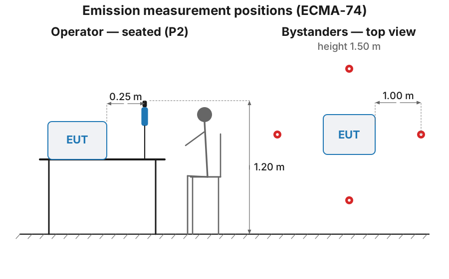
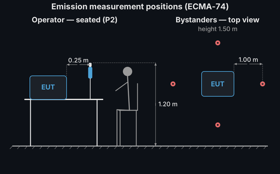
2. Where to measure (ECMA-74) and practice

ECMA-74 (which delegates its tone assessments to ECMA-418-1) also fixes where to measure around a device (context only): phonometry implements the ECMA-418-1 assessments, not the ECMA-74 Annex D measurement procedure:

ECMA-74 emission measurement positions: seated operator microphone at 0.25 m and 1.20 m, and the four bystander positions at 1 m

Proximate secondary tones in the same critical band are combined per clause 11.6; for harmonic complexes assess each component (tone_freq=). Both methods work on Hann-windowed, RMS-averaged spectra and need no absolute calibration (the ratios are level differences).

`tone_to_noise_ratio()` / `prominence_ratio()` parameters

Parameter	Type	Units	Range / default	Notes
`x`	1D array	any (uncalibrated OK)	≥ `fs/resolution_hz` samples	Ratios are level differences: calibration cancels out
`fs`	int	Hz	> 0
`tone_freq`	float, optional	Hz	89.1–11 200; default `None`	`None` assesses the highest peak in the range of interest
`resolution_hz`	float	Hz	> 0; default `1.0`	Tone band must stay within 15 % of the critical band (clause 11.2)

Both return a ToneAssessment(frequency, ratio_db, criterion_db, prominent).

3. Which tonality metric, and when

The library implements four tonality assessments, and they are not interchangeable: each belongs to a different standard with its own purpose, input and output.

	TNR / PR	Tone audibility `ΔL`	Psychoacoustic tonality `T`	Wind-turbine tonal audibility
Standard	ECMA-418-1:2024, clauses 11 and 12	ISO/PAS 20065:2016, adopted by ISO 1996-2:2017 Annex J	ECMA-418-2:2025, clause 6	IEC 61400-11:2012, clause 9.5
Question answered	Is this discrete tone prominent in the emission of a device?	Is the tone audible above the noise that masks it, and by how much?	How tonal does the sound feel?	Is a turbine tone audible at the reference position, wind bin by wind bin?
Input	One FFT spectrum, no calibration needed	Narrow-band spectra with the line spacing declared	The calibrated pressure signal, through the Sottek hearing model	Narrow-band spectra per wind-speed bin, with the reference distance
Output	A ratio in dB against a frequency-dependent criterion, plus a prominent / not prominent verdict	An audibility in dB, whose decisive and mean values feed the tonal adjustment `Kt`	A tonality in `tu_HMS`, a perceptual magnitude with no criterion	An audibility in dB per bin, reported with the turbine’s sound power
Use it for	Declaring ITT equipment emission (ECMA-74 Annex D)	Environmental-noise rating: justifying, or refusing, a tonal penalty	Sound-quality work: comparing designs, not passing a limit	Type testing and acceptance of wind turbines

Read the table as a decision: the purpose of the report picks the metric, not the convenience of the input. A device emission declaration is an ECMA-418-1 prominence verdict; a complaint about a tone from an installation is an ISO 1996-2 rating, so it needs the audibility ΔL that maps to Kt (the tone-audibility guide); a product comparison where nobody is being fined is where the ECMA-418-2 tonality earns its place, because it is a magnitude rather than a threshold test (the sound-quality guide); and a turbine is its own regime, with a measurement procedure in IEC 61400-11 that fixes the geometry and the wind bins (the wind-turbine guide).

Two consequences worth keeping in mind. First, the numbers do not convert: a TNR of 12 dB is not an audibility of 12 dB, because the masking model, the band definition and the reference differ. Second, the metrics can disagree about the same sound, and legitimately so. A tone can be prominent by ECMA-418-1 in the near field of the machine and inaudible at the dwelling where the ISO 1996-2 assessment is made, while a hearing-model tonality stays moderate throughout because it rates the whole sound and not one spectral line. Report the metric the assessment calls for, and quote any other only as supporting evidence.

What this guide covers

Covered. ECMA-418-1:2024 (3rd edition): the tone-to-noise ratio (clause 11, Formulae 9 to 12) and prominence ratio (clause 12, Formulae 23 to 26) methods on Hann-windowed, RMS-averaged spectra, the clause 10 critical-band model, the frequency-dependent prominence criteria, and the clause 11.6 combination of secondary tones sharing a band, all through tone_to_noise_ratio() and prominence_ratio().

Not covered. The prominent verdict these functions return is the numeric criterion only. The standard also requires a prominent tone to be confirmed by aural examination (clauses 11.8/12.8) and to pass the clause 8/9 lower-threshold-of-hearing screen, which needs calibrated absolute levels: both checks are left to the caller. ECMA-74:2025 is covered only as the standard that delegates its tone assessments to ECMA-418-1; its own Annex D measurement procedure and operator/bystander positions (shown above for context) are not implemented here.

References

Ecma International. (2024). Psychoacoustic metrics for ITT equipment — Part 1: Prominent discrete tones (ECMA-418-1:2024 (3rd ed.)). The implemented standard, freely downloadable (the linked PDF is the free download): the tone-to-noise ratio (clause 11) and prominence ratio (clause 12) methods, the critical-band model and the frequency-dependent prominence criteria of section 1.
Ecma International. (2025). Measurement of airborne noise emitted by information technology and telecommunications equipment (ECMA-74:2025 (22nd ed.)). The parent emission standard, freely downloadable (the linked PDF is the free download): the operator/bystander measurement positions of section 2, with Annex D delegating the tone assessments to ECMA-418-1.

Created and maintained byJosé Manuel Requena Plens· GitHub· PyPI· All projects