Acoustic Materials

Characterising an absorber or a partition is a laboratory exercise with three distinct instruments behind it. The reverberation room delivers a spectrum of sound-absorption coefficients that ISO 11654 collapses into a single rated number ${\alpha }_w$ with a letter class. The flow rig (steady or oscillating) measures how hard air is to push through a porous sample, the airflow resistance that governs its low-frequency behaviour (ISO 9053-1/-2). And the impedance tube recovers, at normal incidence, the full complex surface impedance, reflection factor and absorption of a small sample, and, with four microphones, its transmission loss (ISO 10534-1/-2, ASTM E2611). This page covers all three.

1. Sound-absorption rating (ISO 11654)

ISO 354 measures the sound-absorption coefficient ${\alpha }_s$ of a material in one-third-octave bands in a reverberation room. ISO 11654:1997 turns that spectrum into a single-number rating comparable across products.

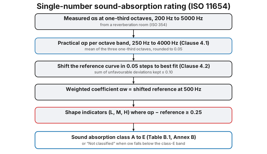
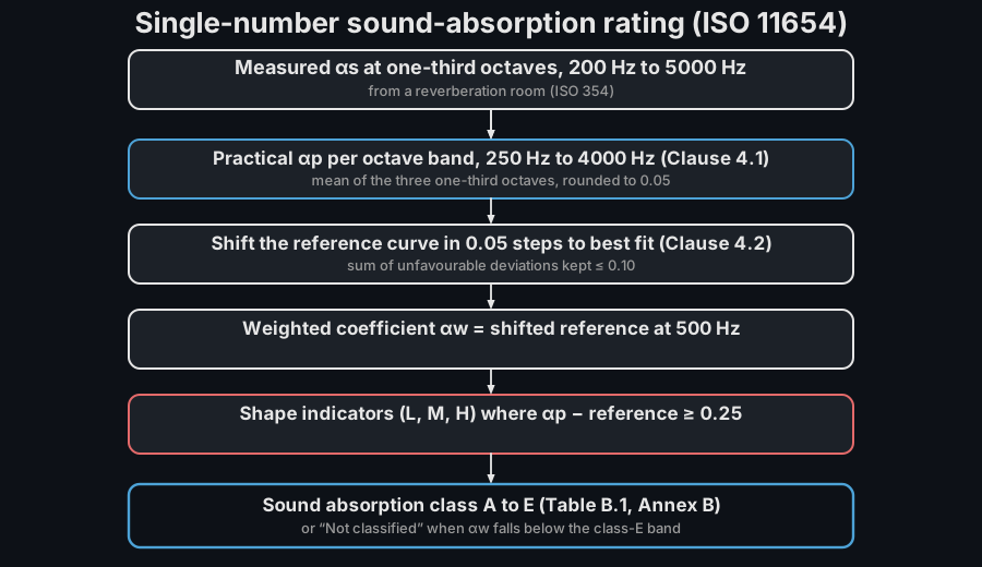
Practical absorption coefficient (Clause 4.1). The one-third-octave data are first grouped into octave bands, each the arithmetic mean of its three thirds:

$${\alpha }_{p,i}=\frac{1}{3}({\alpha }_{i1}+{\alpha }_{i2}+{\alpha }_{i3}),$$

evaluated to the second decimal and then rounded in steps of $0.05$ (the Clause 4.1 NOTE fixes the rounding, e.g. $0.92\to 0.90$); rounded means above $1.00$ are set to $1.00$. The five rating bands are 250, 500, 1000, 2000 and 4000 Hz.

Weighted absorption (Clause 4.2). A fixed reference curve $\{250:0.80,500:1.00,1000:1.00,2000:1.00,4000:0.90\}$ is shifted downwards, towards the measured ${\alpha }_p$, in steps of $0.05$ until the sum of the unfavourable deviations (taken only where the measurement lies below the shifted curve, with magnitude $(\text{curve}-\text{measured})$) is no more than $0.10$. The weighted coefficient ${\alpha }_w$ is the shifted-curve value read at 500 Hz.

Shape indicators (Clause 4.3). When a practical coefficient exceeds the shifted curve by $0.25$ or more, a shape indicator is appended: L at 250 Hz, M at 500 or 1000 Hz, H at 2000 or 4000 Hz (e.g. 0.60(M)).

Absorption class (Table B.1). Finally ${\alpha }_w$ maps to a class: A (0.90–1.00), B (0.80–0.85), C (0.60–0.75), D (0.30–0.55), E (0.15–0.25), or “not classified” (0.00–0.10). Because ${\alpha }_w$ is always a multiple of $0.05$ these ranges partition the grid exactly.

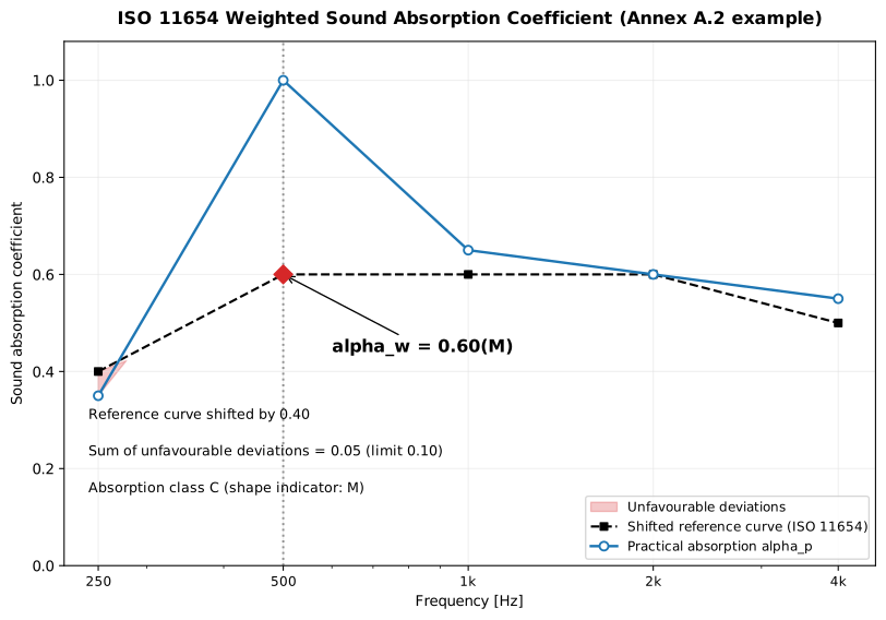
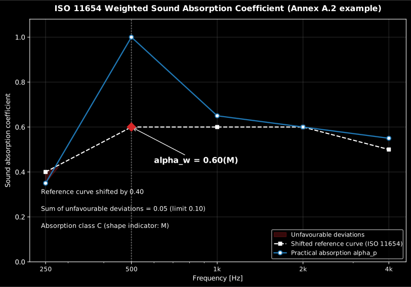
The Annex A.2 worked example: the reference curve is shifted down by 0.40 until the unfavourable deviations sum to 0.05 (≤ 0.10), giving ${\alpha }_w=0.60$; the 500 Hz peak overshoots the shifted curve by ≥ 0.25, adding the M indicator, so the rating is $0.60(\text{M})$, class C.

Show the code for this figure

import matplotlib.pyplot as plt
from phonometry import materials

# ISO 11654 Annex A.2 practical coefficients at 250/500/1000/2000/4000 Hz
result = materials.weighted_absorption([0.35, 1.00, 0.65, 0.60, 0.55])
result.plot()   # practical curve vs shifted reference, deviations shaded
plt.show()

from phonometry import materials

# ISO 11654 Annex A.2 practical coefficients at 250/500/1000/2000/4000 Hz
alpha_p = [0.35, 1.00, 0.65, 0.60, 0.55]

result = materials.weighted_absorption(alpha_p)
print(result.rating_label)          # 0.60(M)
print(result.alpha_w)               # 0.6
print(result.absorption_class)      # C
print(round(result.unfavourable_sum, 2))  # 0.05
result.plot()   # the figure above: practical curve vs shifted reference

# A bare alpha_w also maps straight to its class (Table B.1)
print(materials.absorption_class(0.85))       # B

weighted_absorption accepts the five octave-band ${\alpha }_p$ values (as a sequence or a {frequency: value} mapping); pass the fifteen one-third-octave ${\alpha }_s$ values to practical_absorption_coefficient first if you are starting from raw ISO 354 data. To keep the one-third-octave ${\alpha }_s$ on the result (so the fiche can print the full table every accredited ISO 354 certificate carries), rate it in one step with weighted_absorption_from_third_octave(alpha_s), which forms ${\alpha }_p$, rates it and retains the input ${\alpha }_s$ and its band centres (third_octave_alpha_s, third_octave_bands). The result carries the shifted reference curve and the per-band deviations, and its .plot() renders the figure above.

from phonometry import materials

# Fifteen one-third-octave alpha_s (200 Hz to 5000 Hz), as an ISO 354 report gives
alpha_s = [0.30, 0.35, 0.40, 1.00, 1.00, 1.00, 0.62, 0.66, 0.67,
           0.58, 0.60, 0.62, 0.53, 0.55, 0.57]
result = materials.weighted_absorption_from_third_octave(alpha_s)
print(result.rating_label)          # 0.60(M)
print(result.third_octave_alpha_s)  # the input alpha_s, retained for the fiche

ISO 11654 report (.report())

AbsorptionRatingResult.report(path) renders a one-page PDF fiche laid out like an accredited absorption test report (an ISO 354 reverberation-room measurement rated per ISO 11654): a standard-basis line, an optional metadata header block, the octave-band ${\alpha }_p$ table beside the practical-versus-shifted-reference plot (the result’s own .plot()), the boxed ${\alpha }_w$ single number with its absorption class and applied shift, an optional verdict row and a footer with the fixed disclaimer. When the rating was built with weighted_absorption_from_third_octave, the left table becomes the full ISO 354 one-third-octave ${\alpha }_s$ table with the octave ${\alpha }_p$ on the matching rows, exactly as accredited certificates print it. It uses the same ReportMetadata container and rendering engine as the ISO 717 insulation fiche; passing metadata=None produces a lightweight prediction fiche, and a supplied requirement is read as the minimum ${\alpha }_w$ for the PASS/FAIL verdict. Setting verbose=True swaps the two-column table for the ISO 11654 evaluation columns (practical coefficient, shifted reference, unfavourable deviation). Rendering needs reportlab (pip install phonometry[report]); only engine="reportlab" is supported. The fiche renders in English by default; pass language="es" for a Spanish fiche (translated fixed strings and a comma decimal separator), e.g. result.report("alpha_w_fiche_es.pdf", language="es").

from phonometry import materials, ReportMetadata

# Rate from the fifteen one-third-octave alpha_s so the fiche prints the full
# ISO 354 table; materials.weighted_absorption([...]) also works from alpha_p.
alpha_s = [0.30, 0.35, 0.40, 1.00, 1.00, 1.00, 0.62, 0.66, 0.67,
           0.58, 0.60, 0.62, 0.53, 0.55, 0.57]
result = materials.weighted_absorption_from_third_octave(alpha_s)
result.report(
    "alpha_w_fiche.pdf",
    metadata=ReportMetadata(
        specimen="50 mm porous absorber over a 100 mm air gap",
        area=10.8, mounting="Type A (against a rigid wall)",
        measurement_standard="ISO 354",
        temperature=21.4, relative_humidity=54.0,
        laboratory="Phonometry Reference Laboratory",
        requirement=0.55,          # adds the PASS/FAIL verdict row
    ),
)                                  # alpha_w (shape) + absorption class

The example fiche is regenerated with make reports and kept rendered in the repository; click the preview to open the PDF.

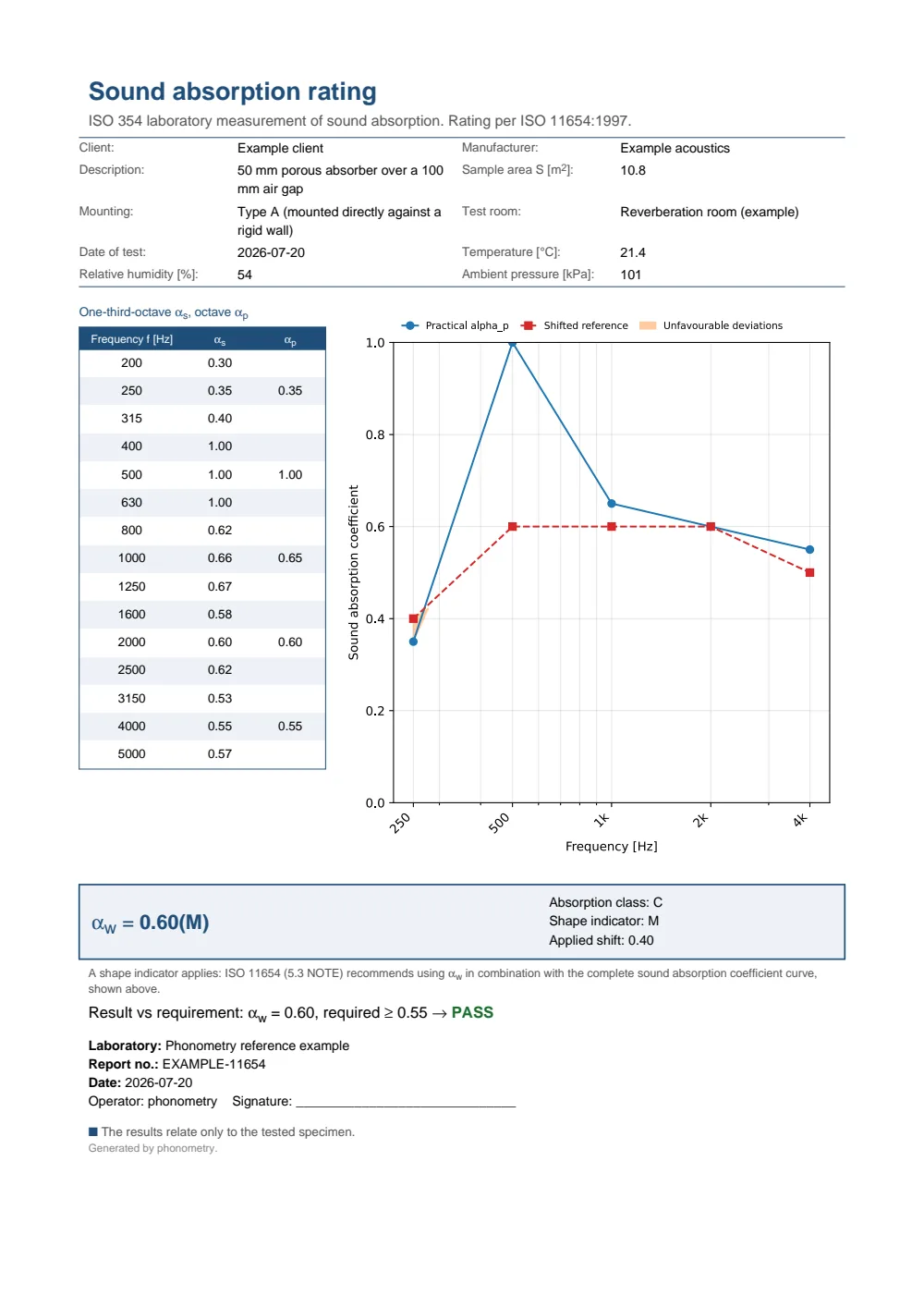
One-page sound absorption fiche: a metadata header (client, specimen, sample area, mounting, reverberation-room temperature, humidity and pressure), the full one-third-octave alpha_s table with the octave alpha_p on the matching rows beside the practical-versus-shifted-reference plot, the boxed alpha_w = 0.60 (M) single-number result with absorption class C and the applied shift, and a PASS verdict against the 0.55 requirement.

Download the report (PDF)

Weighted absorption fiche (AbsorptionRatingResult.report), alpha_w with its class.

ISO 354 measurement (measure_sound_absorption)

The reverberation-room measurement itself is measure_sound_absorption. It takes the one-third-octave reverberation time of the empty room ($T_1$) and of the room with the specimen installed ($T_2$), the room volume $V$ and the specimen area $S$, and returns a frozen SoundAbsorptionMeasurement. The equivalent sound absorption areas follow from Sabine’s equation (ISO 354:2003 Eq. (5)/(7)), $A=55.3V/(cT)-4Vm$, with the speed of sound from Eq. (6), $c=331+0.6t$; the sound absorption coefficient is ${\alpha }_s=(A_2-A_1)/S$ (Eq. (8)/(9)). The coefficient may exceed 1.0 from edge and diffraction effects (Clause 3.7 NOTE 2) and is never clamped. Air attenuation enters only through the per-band coefficient $m$ (default 0, the zero-attenuation reference); pass attenuation_from_alpha of an ISO 9613-1 value when it is needed.

ISO 354 is a characterisation: it produces the ${\alpha }_s$ spectrum, not a single-number rating. The weighted coefficient ${\alpha }_w$ is an ISO 11654 quantity; feed the measured ${\alpha }_s$ to weighted_absorption_from_third_octave above to obtain it.

import numpy as np
from phonometry import materials

freqs = np.array([100, 125, 160, 200, 250, 315, 400, 500, 630, 800,
                  1000, 1250, 1600, 2000, 2500, 3150, 4000, 5000], float)
t_empty = np.array([9.0, 9.0, 8.8, 8.6, 8.4, 8.2, 8.0, 7.8, 7.5, 7.2,
                    6.9, 6.6, 6.2, 5.8, 5.4, 5.0, 4.6, 4.2])
t_specimen = np.array([8.4, 8.2, 7.7, 7.2, 6.5, 5.7, 4.9, 4.2, 3.6, 3.15,
                       2.85, 2.65, 2.55, 2.5, 2.55, 2.6, 2.7, 2.85])

m = materials.measure_sound_absorption(
    freqs, t_empty, t_specimen, volume=200.0, area=10.8, temperature=20.0
)
print(m.alpha_s[7])   # alpha_s at 500 Hz: 0.328...
m.plot()              # alpha_s versus one-third-octave frequency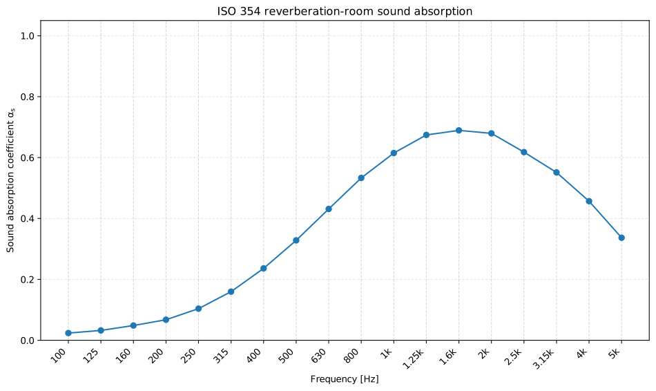

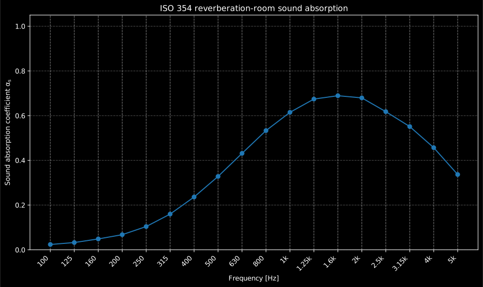
The Sabine inversion of the two decay times: the porous sample barely changes the long low-frequency decays (${\alpha }_s\to 0$), bites hardest where its thickness approaches a quarter wavelength, and eases off at high frequency, a typical thin-porous-absorber signature (Cox & D’Antonio 3e, Ch. 5).

Show the code for this figure

import matplotlib.pyplot as plt
import numpy as np
from phonometry import materials

freqs = np.array([100, 125, 160, 200, 250, 315, 400, 500, 630, 800,
                  1000, 1250, 1600, 2000, 2500, 3150, 4000, 5000], float)
t_empty = np.array([9.0, 9.0, 8.8, 8.6, 8.4, 8.2, 8.0, 7.8, 7.5, 7.2,
                    6.9, 6.6, 6.2, 5.8, 5.4, 5.0, 4.6, 4.2])
t_specimen = np.array([8.4, 8.2, 7.7, 7.2, 6.5, 5.7, 4.9, 4.2, 3.6, 3.15,
                       2.85, 2.65, 2.55, 2.5, 2.55, 2.6, 2.7, 2.85])
m = materials.measure_sound_absorption(
    freqs, t_empty, t_specimen, volume=200.0, area=10.8, temperature=20.0
)

# One line: the alpha_s spectrum over the one-third-octave band axis.
m.plot()
plt.show()

# By hand, from the result's fields:
fig, ax = plt.subplots()
ax.plot(np.arange(freqs.size), m.alpha_s, "o-")
ax.set_xticks(np.arange(freqs.size))
ax.set_xticklabels([f"{f:g}" if f < 1000 else f"{f/1000:g}k" for f in freqs],
                   rotation=45)
ax.set_xlabel("Frequency [Hz]")
ax.set_ylabel("Sound absorption coefficient alpha_s")
plt.show()

ISO 354 report (.report())

SoundAbsorptionMeasurement.report(path) renders a one-page PDF fiche laid out like an accredited reverberation-room absorption test report (ISO 354:2003): a standard-basis line, a metadata header block, the one-third-octave ${\alpha }_s$ table beside the ${\alpha }_s$ curve (the result’s own .plot()), a boxed characterisation headline and a footer with the fixed disclaimer. ISO 354 has no pass/fail verdict and no single-number rating, so the fiche carries neither. Setting verbose=True adds the reverberation times $T_1$/$T_2$ and the equivalent absorption areas $A_1$/$A_2$ to the table.

It uses the same ReportMetadata container and rendering engine as the other fiches. The specimen area $S$, room volume $V$, speed of sound $c$, temperature and humidity are taken from the measurement result (they drove the Sabine inversion); the descriptive ReportMetadata fields that apply here are client, manufacturer, specimen, mounting, test_room, test_date, pressure, measurement_standard, laboratory, operator, report_id and notes. The requirement field is ignored (ISO 354 has no verdict). Rendering needs reportlab (pip install phonometry[report]); only engine="reportlab" is supported. The fiche renders in English by default; pass language="es" for a Spanish fiche (translated fixed strings and a comma decimal separator).

from phonometry import materials, ReportMetadata

m = materials.measure_sound_absorption(
    freqs, t_empty, t_specimen, volume=200.0, area=10.8,
    temperature=20.0, humidity=54.0,
)
m.report(
    "alpha_s_fiche.pdf",
    metadata=ReportMetadata(
        specimen="50 mm porous absorber over a 100 mm air gap",
        mounting="Type A (against a rigid wall)",
        measurement_standard="ISO 354",
        test_room="Reverberation room R1",
        laboratory="Phonometry Reference Laboratory",
    ),
)                                  # one-third-octave alpha_s, 100 Hz to 5000 Hz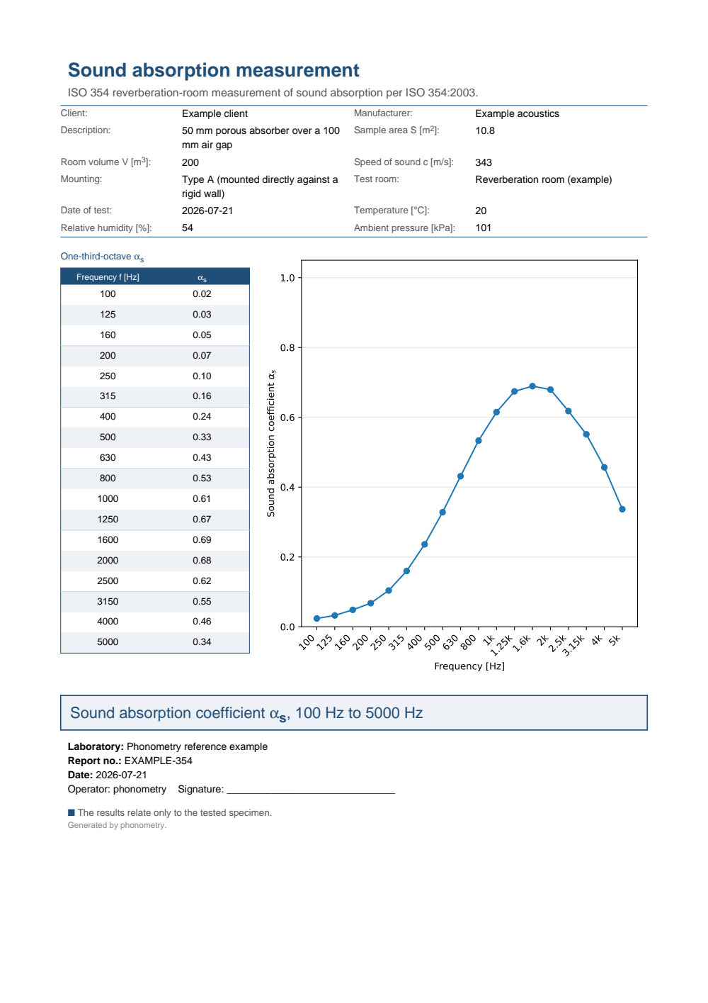

One-page reverberation-room sound absorption fiche: a metadata header (client, specimen, sample area S, room volume V, speed of sound c, mounting, reverberation-room temperature, humidity and pressure), the one-third-octave alpha_s table grouped by octave beside the alpha_s curve, and the boxed characterisation headline over the tested one-third-octave range.

Download the report (PDF)

Reverberation-room absorption fiche (SoundAbsorptionMeasurement.report), the alpha_s spectrum.

2. Airflow resistance (ISO 9053-1/-2)

The airflow resistance quantifies how strongly a porous material opposes a steady or slowly-oscillating flow. Both parts share the same three quantities and units (ISO 9053-1:2018, Clause 3):

$$R=\frac{\Delta p}{q_v}\left[{\text{Pa⋅s/m}}^3\right],R_s=RA\left[\text{Pa⋅s/m}\right],\sigma =\frac{R_s}{d}\left[{\text{Pa⋅s/m}}^2\right],$$

with $\Delta p$ the pressure difference across the specimen, $q_v$ the volumetric flow, $A$ the cross-section and $d$ the thickness. Note the specific airflow resistance $R_s$ is in Pa·s/m (not Pa·s/m²); the airflow resistivity $\sigma$ is $R_s$ per metre of thickness.

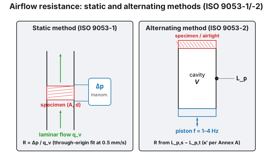
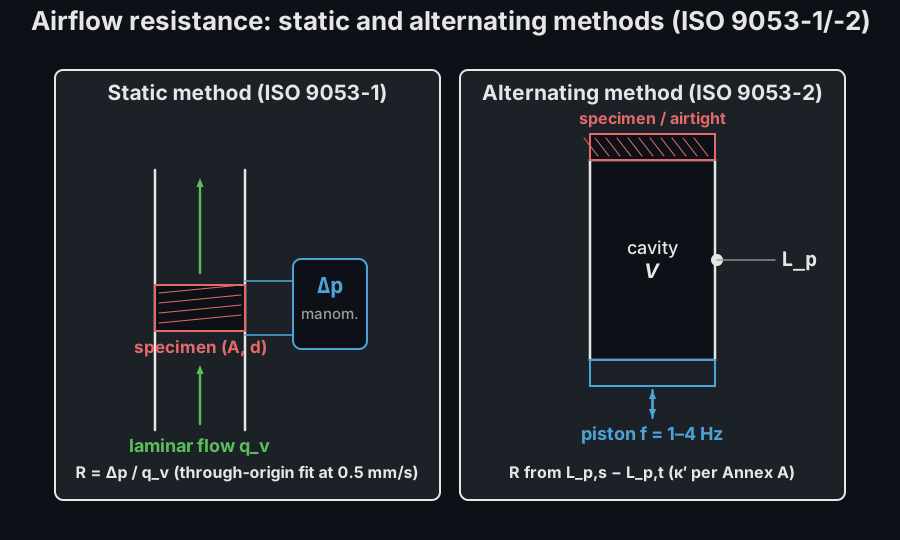
Static method (ISO 9053-1:2018). A steady laminar flow is stepped up and the pressure difference plotted against the linear velocity $u=q_v/A$. A regression of at least second order constrained through the origin, $\Delta p=au+b{u}^2$, is fitted, and $\Delta p$ and $R_s$ are read at the reference velocity $u=0.5\text{mm/s}$ (Clause 7.5); the highest velocity must not exceed 15 mm/s. Because $R_s=\Delta p/u=a+bu$, the linear term $a$ is the zero-velocity specific airflow resistance.

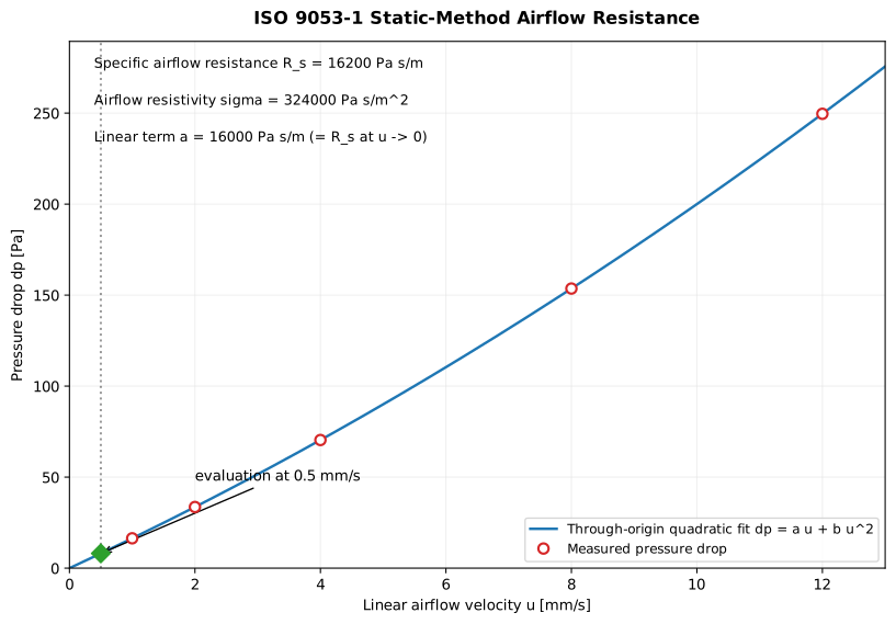
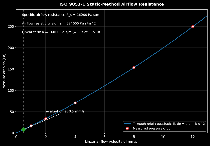
The slightly super-linear pressure drop is fitted through the origin; the specific airflow resistance is the fit read at 0.5 mm/s.

Show the code for this figure

import matplotlib.pyplot as plt
import numpy as np
from phonometry import materials

area = np.pi * 0.05**2                      # 100 mm diameter cell [m^2]
u = np.array([0.5, 1, 2, 4, 8, 12]) * 1e-3  # linear velocity [m/s]
dp = 1.6e4 * u + 4.0e5 * u**2               # measured pressure drop [Pa]
r = materials.static_airflow_resistance(u, dp, area=area, thickness=0.05)

u_fit = np.linspace(0.0, 13e-3, 200)
dp_fit = r.linear_coefficient * u_fit + r.quadratic_coefficient * u_fit**2
fig, ax = plt.subplots()
ax.plot(u_fit * 1e3, dp_fit, label="Through-origin fit  dp = a u + b u^2")
ax.plot(u * 1e3, dp, "o", label="Measured pressure drop")
ax.plot(r.evaluation_velocity * 1e3, r.pressure_drop, "D",
        label="Evaluation at 0.5 mm/s")
ax.set_xlabel("Linear airflow velocity u [mm/s]")
ax.set_ylabel("Pressure drop dp [Pa]")
ax.set_title(f"R_s = {r.specific_resistance:.0f} Pa·s/m")
ax.legend()
plt.show()

import numpy as np
from phonometry import materials

area = np.pi * 0.05**2            # 100 mm diameter cell [m^2]
u = np.array([0.5, 1, 2, 4, 8, 12]) * 1e-3      # linear velocity [m/s]
dp = 1.6e4 * u + 4.0e5 * u**2                    # measured pressure drop [Pa]

r = materials.static_airflow_resistance(u, dp, area=area, thickness=0.05)
print(round(r.specific_resistance))   # 16200   R_s [Pa*s/m]
print(round(r.resistivity))           # 324000  sigma [Pa*s/m^2]
print(round(r.linear_coefficient))    # 16000   a = R_s at u -> 0
r.plot()   # the figure above: the fitted dp(u) with the evaluation point

ISO 9053-1 report (.report())

StaticAirflowResult.report(path) renders a one-page PDF fiche laid out like an accredited airflow-resistance test report (ISO 9053-1:2018, static method): a standard-basis line, an optional metadata header block, a two-panel body with a metrics table (the evaluation velocity, the fitted pressure difference, the airflow resistance $R$, the specific airflow resistance $R_s$, the airflow resistivity $\sigma$ when a thickness is available, and the through-origin fit coefficients $a$ and $b$) beside the fitted $\Delta p(u)$ curve (the result’s own .plot()), the boxed specific airflow resistance $R_s$ with $R$ and $\sigma$ alongside, and a footer with the fixed disclaimer. ISO 9053-1 is a material characterisation, so the fiche carries no pass/fail verdict.

It uses the same ReportMetadata container and rendering engine as the other fiches. The descriptive fields that apply here are client, manufacturer, specimen, thickness (the specimen thickness $d$, in metres, shown in millimetres), test_room, test_date, temperature, relative_humidity, measurement_standard, laboratory, operator, report_id and notes. The requirement field is ignored (ISO 9053-1 has no verdict). The fiche embeds the fitted curve, so rendering needs both reportlab and matplotlib (pip install "phonometry[report,plot]"); only engine="reportlab" is supported. The fiche renders in English by default; pass language="es" for a Spanish fiche (translated fixed strings and a comma decimal separator).

from phonometry import materials, ReportMetadata

r = materials.static_airflow_resistance(u, dp, area=area, thickness=0.05)
r.report(
    "airflow_fiche.pdf",
    metadata=ReportMetadata(
        specimen="50 mm porous absorber (open-cell)",
        thickness=0.050,
        measurement_standard="ISO 9053-1",
        test_room="Static airflow rig, 100 mm cell",
        laboratory="Phonometry Reference Laboratory",
    ),
)                                  # R_s, R and sigma at u = 0.5 mm/s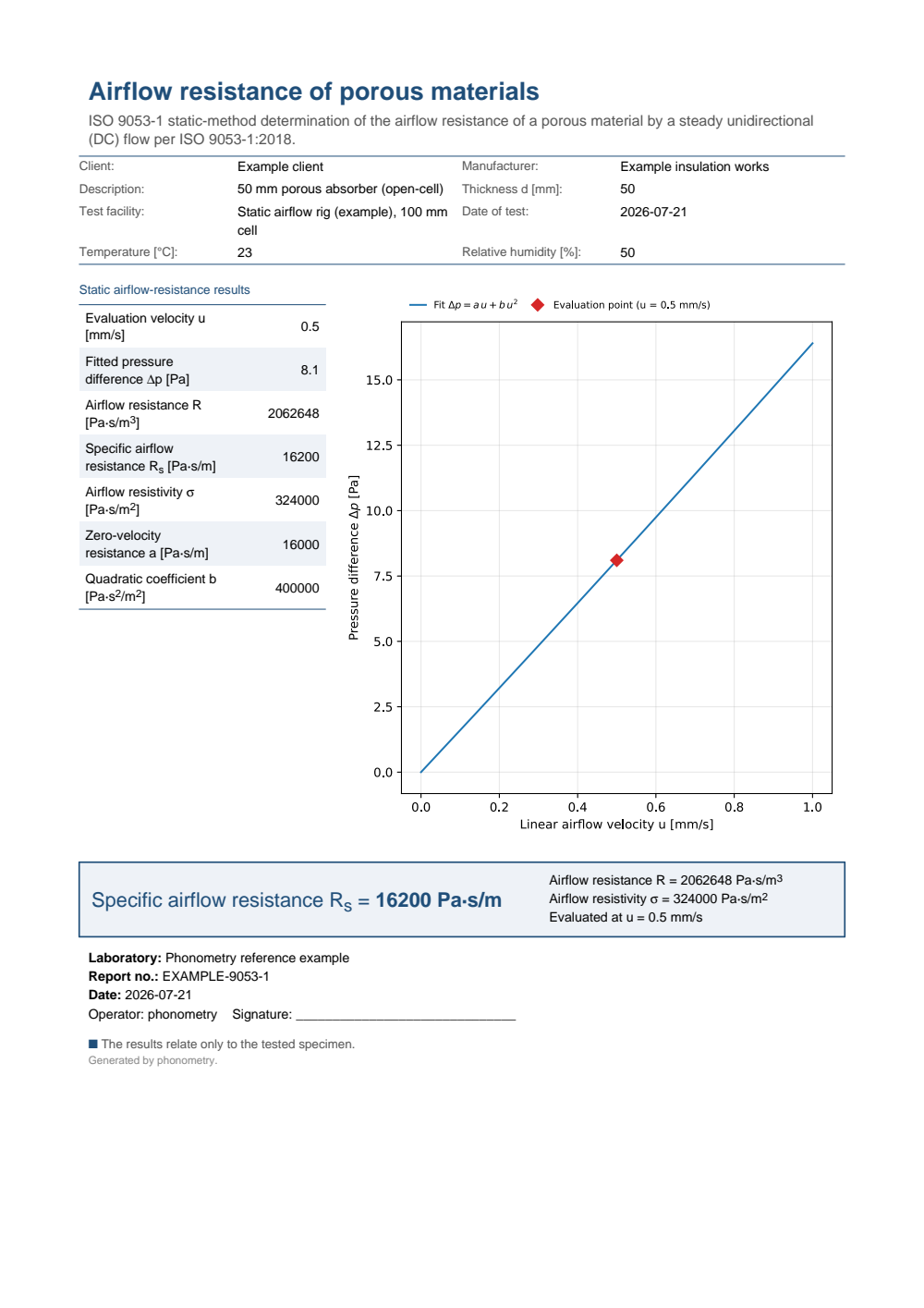

One-page static airflow-resistance fiche: a metadata header (client, manufacturer, specimen, specimen thickness, test facility, temperature and humidity), a metrics table with the evaluation velocity, the fitted pressure difference, the airflow resistance R, the specific airflow resistance R_s, the airflow resistivity sigma and the through-origin fit coefficients a and b beside the fitted pressure-drop curve, and the boxed specific airflow resistance R_s with R and sigma alongside, read at the 0.5 mm/s reference velocity.

Download the report (PDF)

Static airflow-resistance fiche (StaticAirflowResult.report), R_s, R and sigma at 0.5 mm/s.

Alternating method (ISO 9053-2:2020). A piston oscillating at 1–4 Hz drives an alternating flow into a cavity terminated either by the specimen or by an airtight plug; the resistance follows from the sound-pressure-level difference between the two terminations (Formula (2)):

$$R=\frac{{\kappa }^{\prime }{P}_S}{2\pi fV}\cdot \frac{h_t}{h_s}\cdot 10^{(L_{p,s}-L_{p,t})/20},$$

where ${\kappa }^{\prime }$ is the effective ratio of specific heats. Heat conduction between the oscillating air and the cavity walls makes the compression not fully adiabatic; the normative Annex A corrects $\kappa$ down to

$${\kappa }^{\prime }=\frac{\kappa }{\sqrt{1+(\kappa -1)\frac{S}{V}b+\frac{1}{2}((\kappa -1)\frac{S}{V}b{)}^2}},b=\sqrt{\frac{2c_0{l}_h}{\omega }},l_h=\frac{k_a}{{\rho }_0{c}_0{C}_P},$$

with $S$ and $V$ the cavity surface and volume and $b$ the thermal boundary-layer thickness. For the Annex A.3 example cavity this gives ${\kappa }^{\prime }=1.370$, about 2 % below the adiabatic 1.4008.

from phonometry import materials

# Annex A.3 cavity: closed cylinder 100 mm x 100 mm, piston at 2 Hz
kp = materials.effective_kappa(cavity_surface=0.0471, cavity_volume=7.854e-4, frequency=2.0)
print(round(kp, 3))               # 1.37   effective ratio of specific heats

R = materials.alternating_airflow_resistance(
    level_specimen=74.0, level_termination=90.0,
    piston_stroke_specimen=14e-3, piston_stroke_termination=1.4e-3,
    frequency=2.0, cavity_volume=7.854e-4, kappa_prime=kp,
)
print(round(R))                   # 222956  airflow resistance R [Pa*s/m^3]

Pass the effective_kappa result to alternating_airflow_resistance for an Annex-A-conforming figure; its kappa_prime argument otherwise defaults to the uncorrected adiabatic 1.4. The call warns (via AirflowResistanceWarning) when the piston frequency leaves 1–4 Hz or the Formula (3)/(4) validity criteria fail.

3. Impedance tube (ISO 10534-1/-2, ASTM E2611)

The impedance tube measures a small sample at normal incidence. Two standards share the geometry but differ in method and sign convention, so the library keeps their helpers separate and never mixes them.

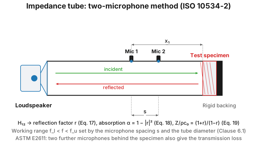
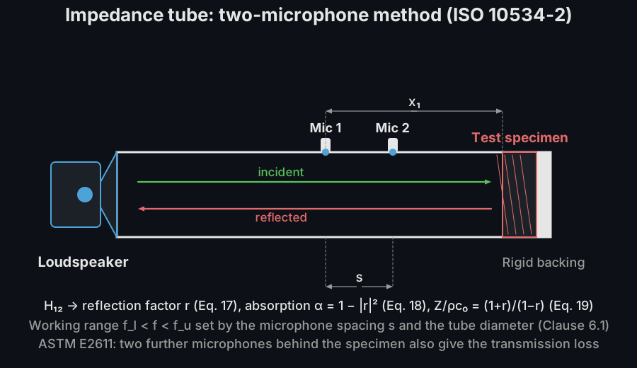
Working frequency range (ISO 10534-2, Clause 4). Everything the tube reports assumes the field inside is a single plane wave, and the geometry sets both ends of the usable band. Above the cut-on of the first cross-sectional mode the field stops being planar: a circular tube of diameter $d$ needs $fd<0.58c_0$ (Eq. (2); $fd<0.50c_0$ for a rectangular tube, Eq. (3)). The microphone spacing $s$ must also stay clear of the half-wavelength singularity of the transfer-function method, $fs<0.45c_0$ (Eq. (4)). At the low end the opposite problem appears: a spacing much shorter than the wavelength leaves almost no phase difference between the microphones to measure, so the Clause 4.2 guideline keeps the spacing above 5 % of the wavelength:

$$\frac{c_0}{20s}<f<\min \left(0.58\frac{c_0}{d},0.45\frac{c_0}{s}\right).$$

No single tube covers the building-acoustics range. A 100 mm tube with a 100 mm spacing works from roughly 170 Hz to 1.5 kHz; reaching the 5 kHz bands takes a small tube (29 mm) with a close spacing, which in turn cannot see the low bands. Laboratories therefore pair a large and a small tube (or one tube with two spacings) and splice the spectra; the two must agree in the overlap bands, and a mismatch there points at the sample cut or mounting, not at the physics.

from phonometry import materials

# A 100 mm tube with 100 mm spacing, and a 29 mm tube with 20 mm spacing.
f_l, f_u = materials.plane_wave_frequency_range(0.100, 343.2, diameter=0.100)
print(round(f_l, 1), round(f_u, 1))     # 171.6 1544.4
f_l, f_u = materials.plane_wave_frequency_range(0.020, 343.2, diameter=0.029)
print(round(f_l, 1), round(f_u, 1))     # 858.0 6864.0

Those limits are easier to see on the hardware itself. plot_impedance_tube_geometry draws a tube to scale with its plane-wave band worked out, and a measured two_microphone_impedance result that was given its geometry (spacing, x1, diameter) redraws its own setup with result.plot_geometry().

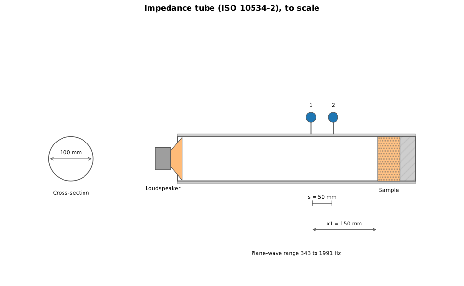
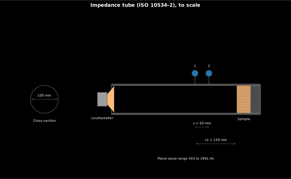
Everything the working-range inequalities talk about, in one to-scale side view: the 100 mm bore sets the 1991 Hz top end, the 50 mm spacing sets the 343 Hz bottom end, and the microphones sit at $s$ = 50 mm with the farther one $x_1$ = 150 mm from the specimen face.

Show the code for this figure

import matplotlib.pyplot as plt
from phonometry import materials

materials.plot_impedance_tube_geometry(spacing=0.05, x1=0.15, diameter=0.10)
plt.show()

# A measured result that retains its geometry draws its own tube:
#   res = materials.two_microphone_impedance(
#       h12, frequency=f, spacing=0.05, x1=0.15, diameter=0.10, ...)
#   res.plot_geometry()

The same helper covers square and rectangular tubes: pass shape="square" or shape="rectangular" and the Eq. (3) factor replaces the circular one, with $d$ the maximum side length. The four-microphone branch keeps its own limits in plane_wave_frequency_range_astm: ASTM E2611 retains the unrounded circular constant ($fd<0.586c$, 6.2.4.1), the same rectangular $fd<0.500c$ (6.2.5), a slightly stricter spacing bound $fs<0.40c$ (6.5.4) and a laxer low end at 1 % of the wavelength (6.2.3). Passing diameter= (and shape=) to two_microphone_impedance, wave_decomposition or the transfer_matrix_* solvers turns the matching check into an advisory warning, and for the Annex A attenuation estimate of a rectangular tube hydraulic_diameter(width, height) supplies the $4A/P$ diameter that tube_attenuation_constant expects.

Standing-wave-ratio method (ISO 10534-1). A probe traverses the standing wave and reads the level difference $\Delta L=L_{\text{max}}-L_{\text{min}}$ between a pressure maximum and the adjacent minimum. The standing-wave ratio, reflection magnitude and absorption follow in closed form:

$$s=10^{\Delta L/20},|r|=\frac{s-1}{s+1},\alpha =1-|r{|}^2.$$

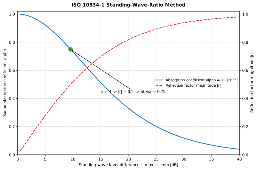
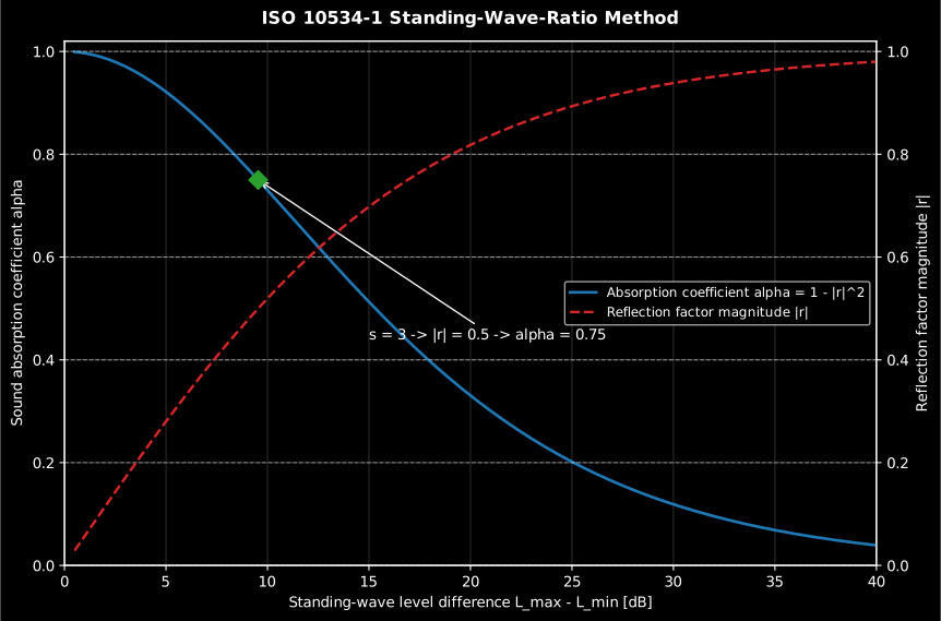
A small level difference means a near-perfect absorber; a level difference of 9.54 dB gives $s=3$, $|r|=0.5$ and $\alpha =0.75$.

Show the code for this figure

import matplotlib.pyplot as plt
import numpy as np
from phonometry import materials

level_diff = np.linspace(0.5, 40.0, 300)    # L_max - L_min [dB]
swr = materials.standing_wave_ratio_from_level(level_diff)
fig, ax = plt.subplots()
ax.plot(level_diff, materials.standing_wave_absorption(swr),
        label="Absorption coefficient alpha")
ax.plot(level_diff, materials.standing_wave_reflection_magnitude(swr), "--",
        label="Reflection factor magnitude |r|")
ax.set_xlabel("Standing-wave level difference L_max - L_min [dB]")
ax.set_ylabel("alpha, |r|")
ax.legend()
plt.show()

from phonometry import materials

s = float(materials.standing_wave_ratio_from_level(9.542))   # level difference [dB] -> SWR
print(round(s, 2))                                  # 3.0
print(round(float(materials.standing_wave_absorption(s)), 2)) # 0.75

Transfer-function method (ISO 10534-2). Two fixed microphones measure the complex transfer function $H_{12}$; from it the reflection factor at the sample face, the absorption and the normalised surface impedance follow (Eqs. (17)–(19)):

$$r=\frac{H_{12}-H_I}{H_R-H_{12}}{e}^{2j{k}_0{x}_1},\alpha =1-|r{|}^2,\frac{Z}{\rho c_0}=\frac{1+r}{1-r},$$

with $H_I=e^{-j{k}_{0}s}$, $H_R=e^{+j{k}_{0}s}$, microphone spacing $s$ and $x_1$ the distance from the sample to the farther microphone.

The incident and reflected waves travel inside a drawn impedance tube and their sum forms the standing-wave envelope; a rigid termination with deep envelope nodes is compared with a porous sample with shallow ones, sampled by the two flush wall microphones.

Download the animation (WebM)

The incident and reflected waves travel inside a drawn impedance tube and their sum forms the standing-wave envelope; a rigid termination with deep envelope nodes is compared with a porous sample with shallow ones, sampled by the two flush wall microphones.

Download the animation (WebM)

import numpy as np
from phonometry import materials

f = np.array([500.0, 1000.0, 1800.0])
x1, spacing, c0 = 0.12, 0.03, 343.2
k0 = materials.tube_wavenumber(f, c0)

# A measured transfer function H12 (here synthesised from r = 0.3 - 0.4j)
target = 0.3 - 0.4j
x2 = x1 - spacing
h12 = (np.exp(1j*k0*x2) + target*np.exp(-1j*k0*x2)) / \
      (np.exp(1j*k0*x1) + target*np.exp(-1j*k0*x1))

r = materials.reflection_factor(h12, spacing=spacing, x1=x1, wavenumber=k0)
print(np.round(materials.absorption_from_reflection(r), 3))     # [0.75 0.75 0.75]
print(np.round(materials.normalized_surface_impedance(r), 2))   # Z / rho c0
# [1.15-1.23j 1.15-1.23j 1.15-1.23j]

The high-level two_microphone_impedance wraps this chain and returns an ImpedanceTubeResult with absorption, reflection factor, surface impedance and normalised impedance, applying the plane-wave frequency-range check and optional tube attenuation; correct any microphone mismatch beforehand with apply_mic_calibration. Its .plot() draws the absorption spectrum $\alpha (f)$ with the reflection-factor magnitude $|r|$ overlaid.

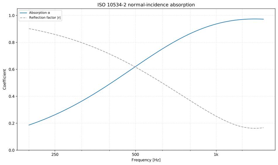
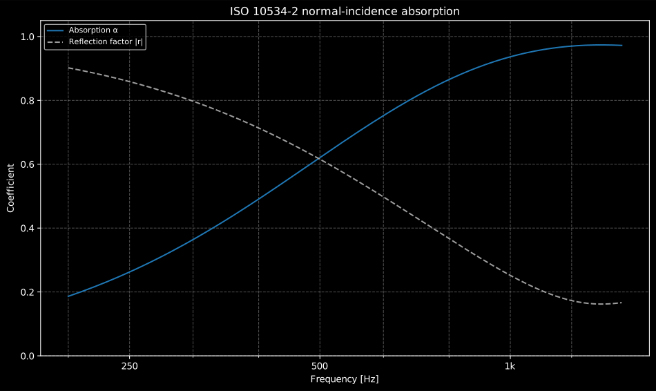
A 50 mm porous absorber measured over the working band of a 100 mm tube: the absorption climbs as the layer thickness grows against the wavelength, and $|r|$ falls as its mirror image ($\alpha =1-|r{|}^2$).

Show the code for this figure

import matplotlib.pyplot as plt
import numpy as np
from phonometry import materials

# A 50 mm porous absorber (Miki, sigma = 20 kPa s/m^2) in a 100 mm tube with
# 100 mm spacing (working band ~170 Hz to 1.5 kHz): the layer model supplies
# the true reflection factor, from which the transfer function H12 follows.
f = np.linspace(200.0, 1500.0, 260)
med = materials.miki(f, 20000.0)
layer = materials.layered_absorber(f, [materials.PorousLayer(0.05, med)])
spacing, x1, c0 = 0.10, 0.20, 343.2
k0 = materials.tube_wavenumber(f, c0)
x2 = x1 - spacing
r_true = layer.reflection
h12 = (np.exp(1j*k0*x2) + r_true*np.exp(-1j*k0*x2)) / \
      (np.exp(1j*k0*x1) + r_true*np.exp(-1j*k0*x1))
result = materials.two_microphone_impedance(
    h12, frequency=f, spacing=spacing, x1=x1, speed_of_sound=c0,
    characteristic_impedance=407.0, diameter=0.10,
)

# One line: alpha(f) with |r| overlaid.
result.plot()
plt.show()

# By hand, from the result's fields:
fig, ax = plt.subplots()
ax.plot(f, result.absorption, label="Absorption alpha")
ax.plot(f, np.abs(result.reflection), "--", label="Reflection factor |r|")
ax.set_xlabel("Frequency [Hz]")
ax.set_ylabel("Coefficient")
ax.legend()
plt.show()

ISO 10534-2 report (.report())

ImpedanceTubeResult.report(path) renders a one-page PDF fiche laid out like an accredited normal-incidence impedance-tube test report (ISO 10534-2:2001): a standard-basis line, a metadata header block, the per-frequency table (the absorption coefficient $\alpha$ and the real and imaginary parts of the normalised surface impedance $z=Z/\rho c_0$) beside the $\alpha (f)$ curve (the result’s own .plot(), on a continuous logarithmic frequency axis), a boxed characterisation headline and a footer with the fixed disclaimer. ISO 10534-2 is a characterisation, so the fiche carries no pass/fail verdict and no single-number rating; the normal-incidence coefficient is not comparable to the random-incidence ${\alpha }_s$/${\alpha }_w$ of ISO 354 / ISO 11654. Setting verbose=True inserts the reflection-factor magnitude $|r|$ column.

It uses the same ReportMetadata container and rendering engine as the other fiches. The measured frequency range is taken from the result; the applicable descriptive and geometric ReportMetadata fields are client, manufacturer, specimen, tube_diameter, tube_shape, mic_spacing, mounting, test_room, test_date, temperature, pressure, measurement_standard, laboratory, operator, report_id and notes (tube_diameter and mic_spacing are given in metres and printed in millimetres). The requirement field is ignored (ISO 10534-2 has no verdict). Rendering needs reportlab (pip install phonometry[report]); only engine="reportlab" is supported. The fiche renders in English by default; pass language="es" for a Spanish fiche (translated fixed strings and a comma decimal separator).

from phonometry import materials, ReportMetadata

result = materials.two_microphone_impedance(
    h12, frequency=freqs, spacing=0.05, x1=0.10,
    speed_of_sound=c0, characteristic_impedance=rho_c, diameter=0.10,
)
result.report(
    "alpha_fiche.pdf",
    metadata=ReportMetadata(
        specimen="Resistive facing over an 86 mm rigidly-backed air cavity",
        tube_diameter=0.10,            # m (printed as 100 mm)
        mic_spacing=0.05,              # m (printed as 50 mm)
        measurement_standard="ISO 10534-2",
        laboratory="Phonometry Reference Laboratory",
    ),
)                       # normal-incidence alpha and impedance over the tube band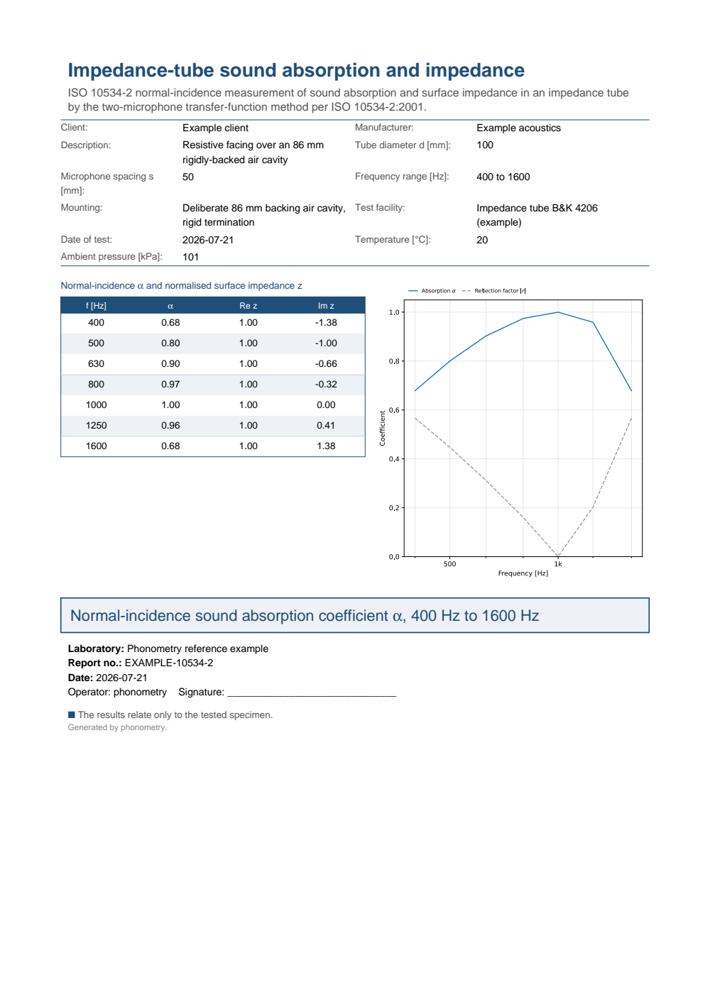

One-page normal-incidence impedance-tube fiche: a metadata header (client, specimen, tube diameter d, microphone spacing s, the measured frequency range, mounting, test facility, temperature and pressure), the per-frequency table of the absorption coefficient alpha and the real and imaginary parts of the normalised surface impedance z beside the alpha curve on a logarithmic frequency axis, and the boxed characterisation headline over the tested frequency range.

Download the report (PDF)

Normal-incidence impedance-tube fiche (ImpedanceTubeResult.report), the alpha spectrum with the surface impedance.

Transmission loss (ASTM E2611). With four microphones (two upstream, two downstream of the sample) a two-load (or one-load) measurement recovers the sample’s transfer matrix, whose entries give the normal-incidence transmission loss, reflection and wavenumber:

$$\mathrm{TL}=20{\log }_{10}\left|\frac{T_{11}+T_{12}/\rho c+\rho c{T}_{21}+T_{22}}{2}\right|.$$

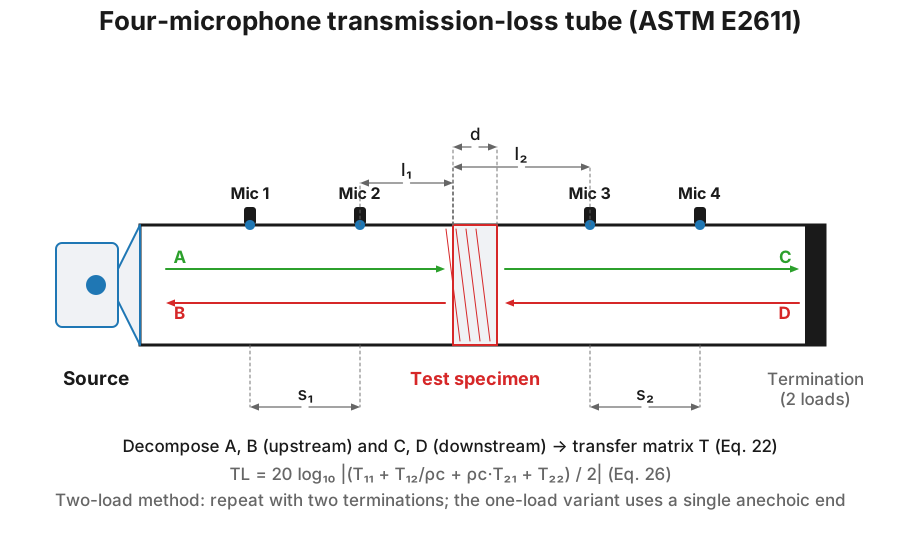
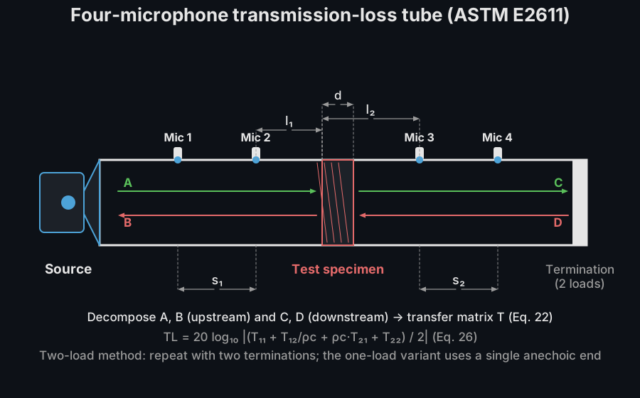
To scale it looks like this. A TransferMatrix recovered by the two-load or one-load solvers retains l1, s1, l2, s2 and the specimen thickness, so tm.plot_geometry() redraws the tube a measurement was taken in.

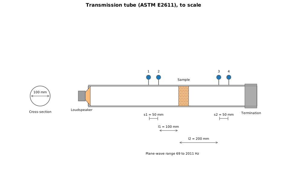
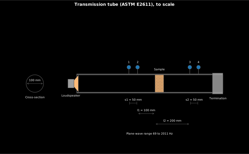
Where the four microphones of the transfer-matrix method actually sit around a 50 mm specimen in a 100 mm tube: $s_1=s_2$ = 50 mm, $l_1$ = 100 mm, $l_2$ = 200 mm, and the changeable termination that provides the second load. The ASTM working range for this geometry is 69 to 2011 Hz.

Show the code for this figure

import matplotlib.pyplot as plt
from phonometry import materials

materials.plot_transmission_tube_geometry(
    l1=0.10, s1=0.05, l2=0.20, s2=0.05, thickness=0.05, diameter=0.10,
)
plt.show()

# A TransferMatrix from transfer_matrix_two_load / _one_load retains its
# geometry, so tm.plot_geometry() redraws the tube it was measured in.

import numpy as np
from phonometry import materials

# An air layer is a known transfer matrix; TL = 0 dB (nothing is lost)
f = np.array([500.0, 1000.0, 2000.0])
k0 = 2*np.pi*f / 343.2
rho_c = 1.186 * 343.2
tm = materials.air_layer_transfer_matrix(thickness=0.05, wavenumber=k0,
                               characteristic_impedance=rho_c)
print(np.round(tm.transmission_loss(rho_c), 6))   # [0. 0. 0.]

transfer_matrix_two_load / transfer_matrix_one_load build the TransferMatrix from the four measured microphone transfer functions (H1, H2, H3, H4) of each load; its methods (transmission_loss, reflection_hard_backed, absorption_hard_backed, characteristic_impedance_material, material_wavenumber) then read off the ASTM E2611 quantities, and its .plot() draws the transmission loss with the hard-backed absorption overlaid (a matrix built by the solvers retains $\rho c$ and, when supplied, the frequency vector, so only a hand-built matrix needs them as arguments). The matrix does not have to come from a measurement: the multilayer solver exposes the chain matrix of any modelled stack in the same convention, so a predicted specimen can be read out exactly like a measured one.

import numpy as np
from phonometry import materials

# The chain matrix of a modelled 50 mm porous layer, read back through the
# ASTM E2611 machinery: TL and hard-backed absorption of the same specimen.
f = np.linspace(200.0, 1600.0, 300)
med = materials.miki(f, 20000.0)
layer = materials.layered_absorber(f, [materials.PorousLayer(0.05, med)])
chain = layer.transfer_matrix                       # shape (2, 2, len(f))
tm = materials.TransferMatrix(t11=chain[0, 0], t12=chain[0, 1],
                              t21=chain[1, 0], t22=chain[1, 1])
print(np.round(float(tm.transmission_loss(407.0)[-1]), 1))   # 9.7 dB at 1.6 kHz
tm.plot(f, 407.0)   # TL(f) with the hard-backed absorption overlaid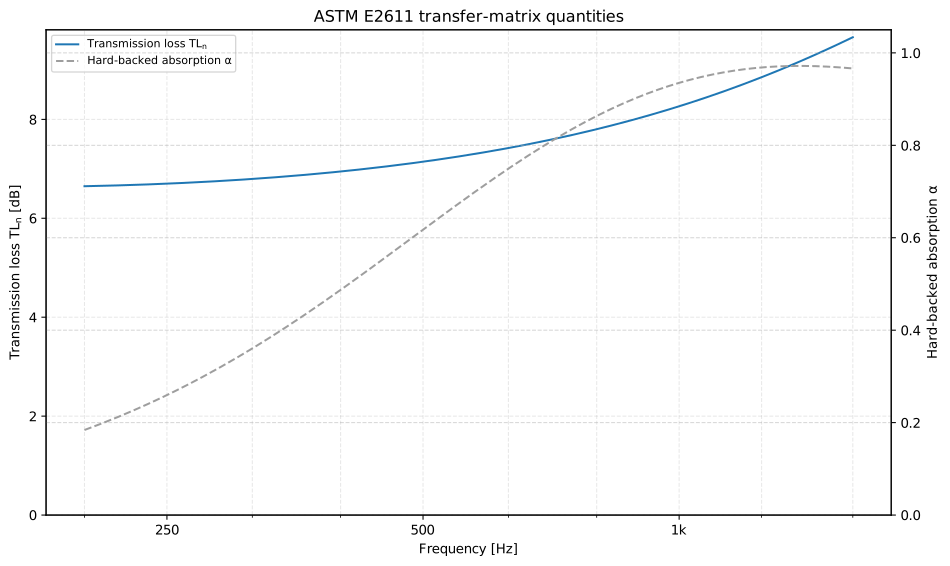

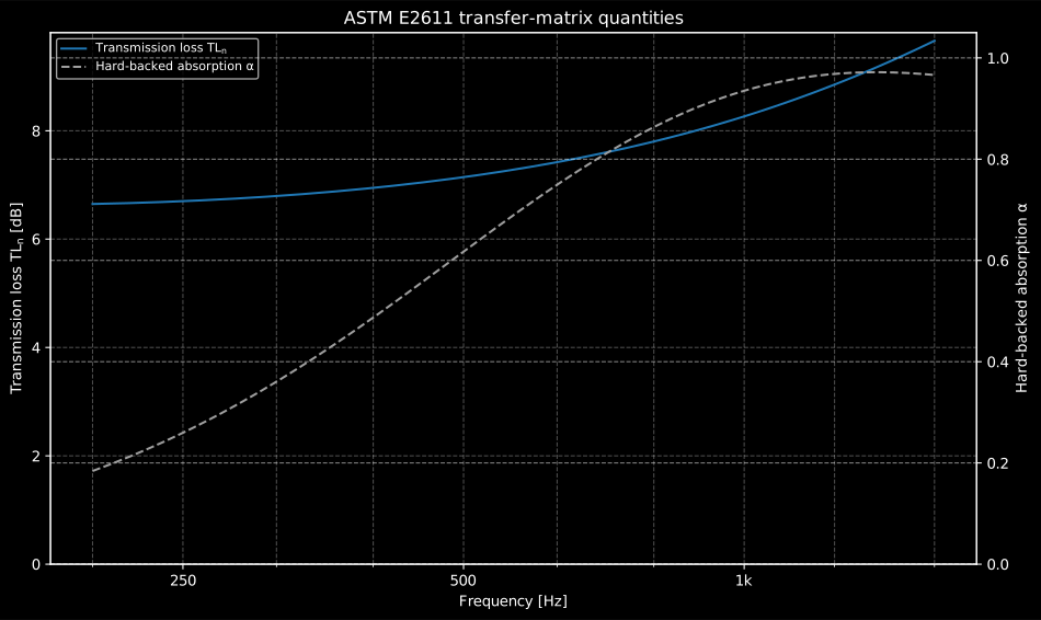
The same four-pole entries answer two different questions: how much sound the free-standing layer lets through (the transmission loss, Eq. (26)) and how much the rigidly-backed layer absorbs (Eq. (28)).

Show the code for this figure

import matplotlib.pyplot as plt
import numpy as np
from phonometry import materials

f = np.linspace(200.0, 1600.0, 300)
med = materials.miki(f, 20000.0)
layer = materials.layered_absorber(f, [materials.PorousLayer(0.05, med)])
chain = layer.transfer_matrix                       # shape (2, 2, len(f))
tm = materials.TransferMatrix(t11=chain[0, 0], t12=chain[0, 1],
                              t21=chain[1, 0], t22=chain[1, 1])

# One line: TL(f) on the left axis, hard-backed absorption on the right.
tm.plot(f, 407.0)
plt.show()

# By hand, from the matrix methods:
fig, ax = plt.subplots()
ax.plot(f, tm.transmission_loss(407.0), label="Transmission loss TL_n")
twin = ax.twinx()
twin.plot(f, tm.absorption_hard_backed(407.0), "--", color="gray",
          label="Hard-backed absorption alpha")
ax.set_xlabel("Frequency [Hz]")
ax.set_ylabel("Transmission loss TL_n [dB]")
twin.set_ylabel("Hard-backed absorption alpha")
plt.show()

Mounting pitfalls. Most bad tube data are made at the sample holder, long before the signal processing. The recurring failures:

• Perimeter gaps. A specimen cut slightly undersize leaves an air sliver along the tube wall. Sound short-circuits around and behind the sample, and the gap itself resonates, so the measured absorption grows a spurious low-to-mid-frequency hump. Cut for a snug slide fit and seal the rim (a thin film of petroleum jelly is the classic remedy) without loading the front face.
• Compression. A specimen cut oversize and forced in is denser than the product it is supposed to represent: the flow resistivity rises, a limp frame is stiffened, and the absorption curve shifts and flattens. The result is repeatable and wrong.
• Hidden back cavity. If the specimen does not sit flush on the rigid backing, the unintended air layer acts as a quarter-wavelength cavity and moves the absorption peak down in frequency, flattering the material. Backing air gaps are perfectly legitimate mountings, but only when they are deliberate, dimensioned and reported with the result.
• Face not plane. A bulging, tilted or torn front face scatters into cross-sectional modes below the nominal cut-on and breaks the normal-incidence assumption the equations rest on. Cut with a sharp tool; do not tear fibrous materials to size.
• One specimen is not the material. Porous products are inhomogeneous at the scale of a tube sample. Measure several cuts and average; a spread between specimens is product variance worth reporting, not measurement noise to hide.

Tube or reverberation room?

The tube and the reverberation room both deliver a number called the “absorption coefficient”, and the two are routinely confused. They are different physical quantities, measured under different sound fields, and they do not match, sometimes not even closely.

The tube measures a normal-incidence coefficient: one plane wave, one angle, a specimen a few centimetres across, and a complex reflection factor that keeps magnitude and phase. ISO 354 measures the random-incidence coefficient ${\alpha }_s$: a diffuse field striking a sample of 10 m² to 12 m² from every direction at once, recovered from the change in the room’s decay time through Sabine’s formula, an energy average with no phase left in it. Because the diffuse field finds more ways into an absorber than the single normal-incidence wave (oblique waves travel a longer path inside the layer), ${\alpha }_s$ usually comes out higher. For a locally reacting surface the two are linked by Paris’ angular average, which defines the statistical absorption coefficient

$${\alpha }_{st}={\int }_0^{\pi /2}\alpha (\theta )\sin 2\theta \mathrm{d}\theta ,$$

an integral that weights the oblique angles most heavily; evaluating it needs the angle-dependent $\alpha (\theta )$ from the measured surface impedance, not just the normal-incidence coefficient itself.

Why ISO 354 values exceed 1. A ratio of absorbed to incident energy cannot exceed one, yet reverberation-room reports of ${\alpha }_s=1.05$ to $1.20$ for thick porous absorbers are routine and correct by the method. Sabine’s formula converts the decay-time change into an equivalent absorption area $A$, and ${\alpha }_s=A/S$ divides by the geometric sample area $S$. Diffraction at the sample edges lets the specimen drain energy from a sound field wider than its footprint (the edge effect), so the equivalent area can exceed the geometric one. Such values are not errors, but they are not portable either: they depend on the sample size and perimeter, which is precisely why ISO 354 fixes both. The ISO 11654 rating simply truncates: practical coefficients above $1.00$ are set to $1.00$ (section 1). Prediction inputs get no such silent clipping in this library: each reverberation-time estimator enforces its own mathematical domain, so Sabine and Eyring accept ISO 354 values at or above one as supplied (Eyring as long as the mean absorption stays below one), while Millington-Sette rejects them (its per-surface logarithm diverges at one) and any adjustment below one is left to the caller. The equivalent-absorption-area budget of EN 12354-6 likewise accepts the coefficients as supplied.

Which to use. They answer different questions. The reverberation-room value is the one that feeds diffuse-field prediction: Sabine reverberation estimates, the equivalent absorption areas of EN 12354-6 and the ${\alpha }_w$ rating and class, all of which expect random incidence over a mounted, finite sample (ISO 354’s Annex B mounting types exist because the mounting is part of the result). The tube value is the laboratory and development tool: it needs only a few square centimetres of material, resolves magnitude and phase, and its surface impedance pins down the parameters of porous-material models in the Allard and Atalla tradition, with the airflow resistivity of section 2 as the first input; the fitted model then predicts the layer at any angle, thickness or backing. What the tube number is not is a drop-in substitute for ${\alpha }_s$: feeding normal-incidence coefficients into a Sabine or EN 12354-6 budget systematically underpredicts the installed absorption.

4. Sound-absorption measurement uncertainty (ISO 12999-2)

A rated absorption coefficient means little without its uncertainty. ISO 12999-2:2020 gives the standard uncertainty $u$ of the quantities produced by a reverberation-room measurement (ISO 354) and its ratings (ISO 11654, EN 1793-1), estimated from inter-laboratory tests to ISO 5725. It is the sound-absorption companion of the sound-insulation uncertainty of ISO 12999-1 (Field Insulation Measurement and Ratings).

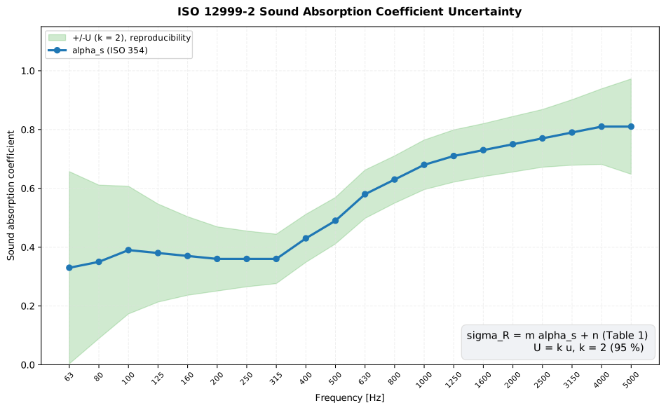
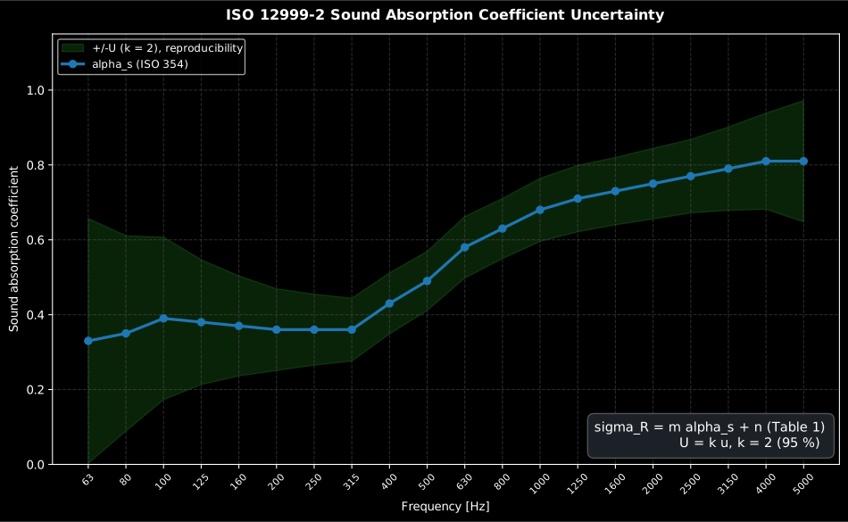
One-third-octave bands (Clause 5). For the sound-absorption coefficient the reproducibility standard deviation is ${\sigma }_R=m{\alpha }_s+n$ (Formula (1)), and for the equivalent absorption area ${\sigma }_R=m{A}_T+nS$ with $S=10{\text{m}}^2$ (Formula (2)), where $m$ and $n$ are the frequency-dependent constants of Table 1 (63–5000 Hz). The repeatability value is ${\sigma }_r=0.6{\sigma }_R$ (Formula (3)).

Practical coefficient (Clause 6). For the ISO 11654 practical coefficient ${\sigma }_R=m{\alpha }_p+n$ in octave bands with the constants of Table 2 (250–4000 Hz); again ${\sigma }_r=0.6{\sigma }_R$.

Single numbers (Clause 7). The weighted coefficient ${\alpha }_w$ has a constant standard uncertainty (${\sigma }_R=0.035$, ${\sigma }_r=0.020$); the EN 1793-1 single-number rating $D{L}_{\alpha ,\text{NRD}}$ scales with the value (${\sigma }_R=0.10D{L}_{\alpha }$, ${\sigma }_r=0.02D{L}_{\alpha }$).

Reporting (Clause 8). The expanded uncertainty is $U=ku$ (Formula (10)) with the Table 3 coverage factor $k$ ($k=2.0$ at 95 %, Gaussian). The reported $U$ is rounded to two decimals for absorption coefficients and one decimal for the equivalent area and $D{L}_{\alpha ,\text{NRD}}$.

Show the code for this figure

import matplotlib.pyplot as plt
from phonometry import materials

# ISO 12999-2 Table 4 worked example: alpha_s per one-third-octave band.
freqs = [63, 80, 100, 125, 160, 200, 250, 315, 400, 500,
         630, 800, 1000, 1250, 1600, 2000, 2500, 3150, 4000, 5000]
alpha_s = [0.33, 0.35, 0.39, 0.38, 0.37, 0.36, 0.36, 0.36, 0.43, 0.49,
           0.58, 0.63, 0.68, 0.71, 0.73, 0.75, 0.77, 0.79, 0.81, 0.81]
result = materials.sound_absorption_coefficient_uncertainty(alpha_s, freqs, confidence=0.95)
result.plot()   # alpha_s with the +/-U (k = 2) reproducibility ribbon
plt.show()

from phonometry import materials

# Reproducibility uncertainty of alpha_s at 1000 Hz (Table 1: m=0.040, n=0.015).
r = materials.sound_absorption_coefficient_uncertainty([0.68], [1000], confidence=0.95)
print(round(float(r.standard_uncertainty[0]), 4))            # 0.0422 (sigma_R)
print(float(r.reported_expanded_uncertainty[0]))             # 0.08  (U, k=2)
r.plot()   # the figure above: alpha_s with its +/-U (k = 2) ribbon

# Single-number ratings (Clause 7 worked examples).
print(float(materials.weighted_coefficient_uncertainty(0.70).reported_expanded_uncertainty[0]))  # 0.07
print(float(materials.single_number_rating_uncertainty(8.1).reported_expanded_uncertainty[0]))   # 1.6

What this guide covers

Covered. ISO 11654:1997’s weighted absorption rating: the practical coefficient of Clause 4.1, the reference-curve shift of Clause 4.2, the shape indicators of Clause 4.3, and the Table B.1 absorption class. These are built by weighted_absorption and weighted_absorption_from_third_octave. The ISO 354:2003 Sabine inversion (Eqs. (5)-(9)) in measure_sound_absorption. Both parts of ISO 9053: the static method of Clause 7.5 (static_airflow_resistance) and the alternating method with the Annex A effective ratio of specific heats (effective_kappa, alternating_airflow_resistance). The impedance-tube trio: the ISO 10534-1 standing-wave-ratio method (standing_wave_ratio_from_level and its companions), the ISO 10534-2 transfer-function method with its Clause 4 frequency-range check (two_microphone_impedance, plane_wave_frequency_range), and the ASTM E2611 four-microphone transfer-matrix method (transfer_matrix_two_load, transfer_matrix_one_load, TransferMatrix). ISO 12999-2:2020’s measurement-uncertainty formulae (Clauses 5-8) for the one-third-octave and practical coefficients and for the single-number ratings, in sound_absorption_coefficient_uncertainty, weighted_coefficient_uncertainty and single_number_rating_uncertainty.

Not covered. The statistical (random-incidence) absorption coefficient ${\alpha }_{st}$ of Paris’ angular average is described but not computed: it needs the angle-dependent $\alpha (\theta )$ from the surface impedance, which nothing here derives. Two editions cited only as later revisions are not implemented: ISO 10534-2:2023 (the code follows the 1998/2001 transfer-function method) and ASTM E2611-24 (the code follows E2611-19). ISO 10534-1:1996 is implemented as its European adoption BS EN ISO 10534-1:2001, not read directly from the 1996 ISO text. ISO 12999-2’s uncertainty formula for the EN 1793-1 single-number rating $D{L}_{\alpha ,\text{NRD}}$ is implemented, but EN 1793-1’s own in-situ measurement method (road-traffic noise-reducing devices) is not.

See also

• API reference: materials.impedance_tube, materials.airflow_resistance and materials.absorption_uncertainty.

References

• Allard, J. F., & Atalla, N. (2009). Propagation of sound in porous media: Modelling sound absorbing materials (2nd ed.). Wiley. https://doi.org/10.1002/9780470747339The porous-material theory behind the measured quantities: airflow resistivity as a model input, and the surface impedance and absorption the tube recovers. ISBN 978-0-470-74661-5.
• ASTM International. (2019). Standard test method for normal incidence determination of porous material acoustical properties based on the transfer matrix method (ASTM E2611-19). The four-microphone transfer-matrix method behind the transmission-loss helpers. The edition implemented here; since revised as ASTM E2611-24 (https://store.astm.org/e2611-24.html).
• Cox, T. J., & D'Antonio, P. (2017). Acoustic absorbers and diffusers: Theory, design and application (3rd ed.). CRC Press. https://doi.org/10.1201/9781315369211Absorber measurement and design in practice: the tube and room methods side by side, mountings, and the edge-effect discussion behind the tube-or-reverberation-room section. ISBN 978-1-4987-4099-9.
• International Organization for Standardization. (1996). Acoustics — Determination of sound absorption coefficient and impedance in impedance tubes — Part 1: Method using standing wave ratio (ISO 10534-1:1996). The standing-wave-ratio method of section 3; the edition implemented here is its European adoption BS EN ISO 10534-1:2001.
• International Organization for Standardization. (1997). Acoustics — Sound absorbers for use in buildings — Rating of sound absorption (ISO 11654:1997). The weighted sound-absorption rating of section 1: the practical coefficient, the shifted reference curve, the shape indicators and the absorption class, validated against the standard's own Annex A worked example.
• International Organization for Standardization. (1998). Acoustics — Determination of sound absorption coefficient and impedance in impedance tubes — Part 2: Transfer-function method (ISO 10534-2:1998). The two-microphone transfer-function method and its plane-wave frequency-range limits. Adopted in Europe as EN ISO 10534-2:2001, the edition implemented here; since revised as ISO 10534-2:2023 (https://www.iso.org/standard/81294.html).
• International Organization for Standardization. (2003). Acoustics — Measurement of sound absorption in a reverberation room (ISO 354:2003). The reverberation-room method that produces the alpha_s spectra rated by ISO 11654, including the Annex B specimen mountings.
• International Organization for Standardization. (2018). Acoustics — Determination of airflow resistance — Part 1: Static airflow method (ISO 9053-1:2018). The static method of section 2, with the through-origin regression and the 0.5 mm/s reference velocity.
• International Organization for Standardization. (2020). Acoustics — Determination and application of measurement uncertainties in building acoustics — Part 2: Sound absorption (ISO 12999-2:2020). The sound-absorption measurement uncertainty of section 4, validated against the standard's own worked examples (Tables 4/5).
• International Organization for Standardization. (2020). Acoustics — Determination of airflow resistance — Part 2: Alternating airflow method (ISO 9053-2:2020). The alternating method of section 2, with the Annex A effective ratio of specific heats, validated against the standard's own Annex A.3 worked example.