Predicting Panel Sound Insulation

A laboratory test measures the sound reduction index $R$ of a finished element; this page instead predicts $R(f)$ from the physical properties of the construction, so a partition can be designed before it is built. It covers the airborne insulation of a single panel (the mass law and the coincidence dip), the double wall (its mass-spring-mass resonance), the transmission through slits and apertures that caps any real construction, the radiation efficiency of a bending plate, and the point mobilities that set the vibrational power a structure absorbs. The measured counterparts these predictions feed live in Predicting Sound Insulation (EN 12354) and Field Insulation Measurement and Ratings.

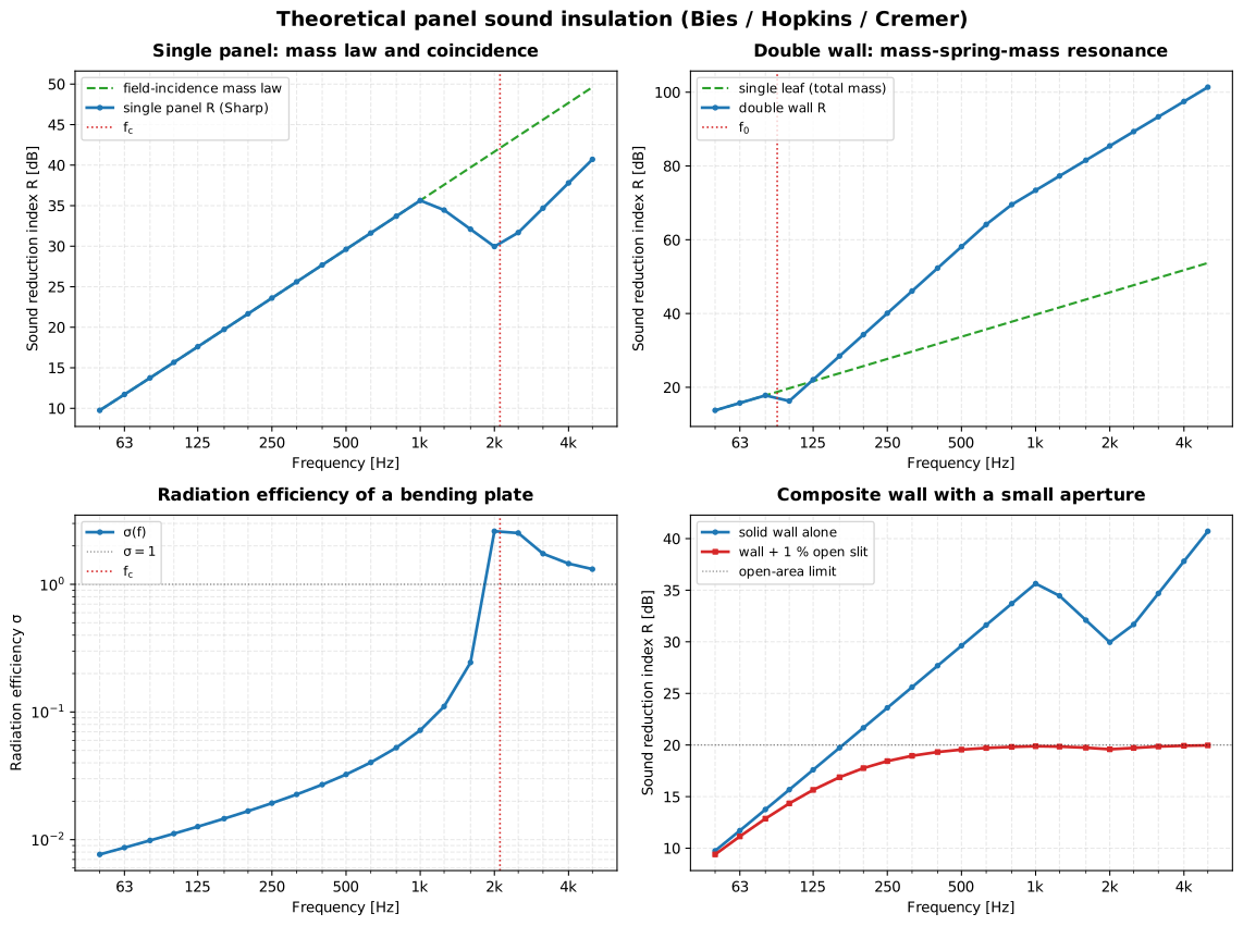
Single panel: the mass law and coincidence (Bies 7.2)

A limp, non-stiff panel transmits sound by being driven bodily by the incident pressure; the heavier it is and the higher the frequency, the more it resists. The normal-incidence mass law (Bies Eq. 7.40) and its diffuse-field form (Eq. 7.42) are

$$T{L}_0=10{\log }_{10}\left[1+{\left(\frac{\pi f{m}^{\prime \prime }}{{\rho }_0{c}_0}\right)}^2\right],TL=T{L}_0-{\Delta }_{\text{band}},$$

with $m^{\prime \prime }$ the mass per unit area and ${\Delta }_{\text{band}}=5.5$ dB (one-third octave) or $4.0$ dB (octave). Above the argument’s knee the mass law rises 6 dB per octave and 6 dB per doubling of mass, the two facts every insulation calculation rests on.

A real panel is also stiff, so at the coincidence (critical) frequency (Bies Eq. 7.3)

$$f_c=\frac{c_0^2}{2\pi }\sqrt{\frac{m^{\prime \prime }}{B^{\prime }}}=\frac{0.55c_0^2}{c_{L}h},$$

the free bending wavelength matches the trace wavelength of the incident sound and the panel goes transparent: the coincidence dip. Sharp’s method holds the field-incidence mass law up to $f_c/2$, drops through a straight line in $\log f$, and from $f_c$ upward follows (Eq. 7.44) $TL=10\lg [1+(\pi f{m}^{\prime \prime }/{\rho }_0{c}_0{)}^2]+10\lg (2\eta f/\pi f_c)$ with the loss factor $\eta$. The dip sits at Bies design-chart point B, $TL=20\lg (f_c{m}^{\prime \prime })+10\lg \eta -44$.

import numpy as np
from phonometry import (
    coincidence_frequency, plate_bending_stiffness,
    single_panel_transmission_loss,
)

# 6 mm float glass: E = 62 GPa, rho = 2500 kg/m3, nu = 0.24, eta = 0.024.
bands = np.array([100, 125, 160, 200, 250, 315, 400, 500, 630, 800,
                  1000, 1250, 1600, 2000, 2500, 3150], dtype=float)
mass = 2500.0 * 0.006                                 # 15 kg/m2
bp = plate_bending_stiffness(6.2e10, 0.006, 0.24)     # B' [N.m]
fc = coincidence_frequency(mass, bp)
print(round(fc))                                      # 2107 Hz (Hopkins declares ~2079)

res = single_panel_transmission_loss(bands, mass, critical_frequency=fc,
                                     loss_factor=0.024)
print(round(res.rating().rating))                     # 32  ->  Rw = 32 dB (catalogue 6 mm glass)

res.plot()   # predicted R(f) with the critical frequency marked (needs matplotlib)

The predicted spectrum plugs straight into the ISO 717-1 rating through res.rating(), and into EN 12354 as the “predicted” element $R$ where the standard would otherwise demand a laboratory measurement.

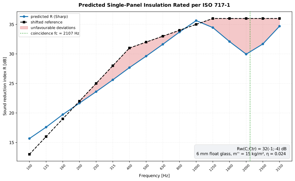
The predicted Sharp spectrum rated exactly like a measurement: the coincidence dip at $f_c\approx 2.1$ kHz collects most of the unfavourable deviations, and the shifted reference read at 500 Hz gives the catalogue $R_w=32$ dB of 6 mm glass.

Show the code for this figure

import matplotlib.pyplot as plt
import numpy as np
from phonometry import (
    coincidence_frequency, plate_bending_stiffness,
    single_panel_transmission_loss,
)

# 6 mm float glass: E = 62 GPa, rho = 2500 kg/m3, nu = 0.24, eta = 0.024.
bands = np.array([100, 125, 160, 200, 250, 315, 400, 500, 630, 800,
                  1000, 1250, 1600, 2000, 2500, 3150], dtype=float)
mass = 2500.0 * 0.006
bp = plate_bending_stiffness(6.2e10, 0.006, 0.24)
fc = coincidence_frequency(mass, bp)
res = single_panel_transmission_loss(bands, mass, critical_frequency=fc,
                                     loss_factor=0.024)
w = res.rating()

# One line each — the predicted R(f), or the rated curve vs the reference:
res.plot()
w.plot()
plt.show()

# By hand, combining both on one axes:
fig, ax = plt.subplots()
ax.semilogx(bands, res.transmission_loss, "o-", label="predicted R (Sharp)")
ax.semilogx(w.band_centers, w.shifted_reference, "s--",
            label="shifted reference")
ax.fill_between(w.band_centers, w.measured, w.shifted_reference,
                where=w.measured < w.shifted_reference, interpolate=True,
                alpha=0.3, label="unfavourable deviations")
ax.axvline(fc, ls=":", color="tab:green", label=f"fc = {fc:.0f} Hz")
ax.set_xlabel("Frequency [Hz]")
ax.set_ylabel("Sound reduction index R [dB]")
ax.set_title(f"Rw = {w.rating} dB  (C={w.c:+d}; Ctr={w.ctr:+d})")
ax.legend()
plt.show()

Double wall: the mass-spring-mass resonance (Bies 7.2.6)

Two leaves separated by a cavity behave as a mass-spring-mass system, with the cavity air (or fill) the spring. Below its resonance (Bies Eq. 7.62, Hopkins Eq. 4.73)

$$f_0=\frac{1}{2\pi }\sqrt{\frac{s^{\prime \prime }(m_1+m_2)}{m_1{m}_2}}=60\sqrt{\frac{m_1+m_2}{m_1{m}_{2}d}}\text{(empty air gap)},$$

the pair moves as one and follows the mass law of the combined mass; above it the two mass laws add, boosted by the cavity, until the limiting frequency $f_l=c_0/(2\pi d)$ where the boost saturates at 6 dB (Eq. 7.64). A porous fill (any PorousMediumResult) softens the cavity and lowers $f_0$.

from phonometry import double_wall_transmission_loss, mass_spring_mass_resonance
from phonometry import mass_law_transmission_loss, miki

# Two 12 kg/m2 leaves, 75 mm air gap.
f0 = mass_spring_mass_resonance(12.0, 12.0, 0.075)
print(round(f0))                                          # 89 Hz

# Below f0 the double wall equals the mass law of the total mass 24 kg/m2:
dw = double_wall_transmission_loss(bands, 12.0, 12.0, 0.075)
print(round(float(dw.transmission_loss[0]), 1),
      round(float(mass_law_transmission_loss(bands[0], 24.0)), 1))   # equal

# A mineral-wool fill (a materials porous model) lowers the resonance:
fill = miki([f0], 7000.0)
print(round(mass_spring_mass_resonance(12.0, 12.0, 0.075, cavity_medium=fill)))  # < 89 Hz

dw.plot()   # double-wall R(f) with the mass-spring-mass resonance marked (needs matplotlib)

Slits, holes and apertures (Hopkins 4.3.10)

A small air path is the real limit on any heavy construction. The transmission coefficient of a straight slit (Gomperts, Hopkins Eq. 4.99) and of a circular hole (Wilson & Soroka, Eq. 4.102) are predicted directly, with the slit’s resonances at $d+2e=z\lambda /2$ (Eq. 4.101). They combine with the wall in the area-weighted energy sum (Eq. 4.92)

$$R=-10{\log }_{10}\left(\frac{1}{{\sum }_n{S}_n}\sum _n{S}_{n}10^{-R_n/10}\right),$$

so a bare opening of relative area $S_a/S$ caps the composite at $10\lg (S/S_a)$; a 1 % opening can never do better than 20 dB, whatever the wall.

from phonometry import (
    composite_transmission_loss, slit_transmission_coefficient,
    slit_resonance_frequencies,
)

# A 2 mm x 100 mm-deep slit: its transmission peaks at the half-wavelength
# resonances of the slit depth.
print(slit_resonance_frequencies(0.1, 0.002, orders=2).round().tolist())   # [~1500, ~3100]

# A wall of Rw = 50 dB with 1 % of its area left open as a slit is capped:
print(round(float(composite_transmission_loss([0.99, 0.01], [50.0, 0.0])), 1))   # 20.0

Radiation efficiency of a bending plate (Hopkins 2.9)

How much airborne power a vibrating plate actually radiates per unit mean-square velocity is its radiation efficiency $\sigma$, the radiation factor $\epsilon$ that Sound Power from Surface Vibration (ISO 7849) otherwise takes as a measured input. Below the critical frequency the plate radiates weakly (edge and corner modes); above it $\sigma \to 1$ (Leppington/Maidanik, Hopkins Eqs 2.227-2.230):

$$\sigma =\frac{1}{\sqrt{1-f_c/f}}(f>f_c),\sigma \to 1.$$

from phonometry import radiation_efficiency, sound_power_from_vibration

# The 6 mm glass pane (1.5 x 1.25 m) of the single-panel example above.
sig = radiation_efficiency(bands, 1.5, 1.25, fc)
print(sig.radiation_efficiency[bands == 2000].round(2))    # ~2.5 (peak at coincidence)

# Feed the prediction straight into ISO 7849 as the radiation factor:
lw = sound_power_from_vibration(velocity_level=80.0, area=1.875,
                                radiation_factor=sig.radiation_efficiency,
                                frequencies=bands)

sig.plot()   # sigma(f) with the coincidence peak (needs matplotlib)

Point mobilities of infinite structures (Cremer Table 5.1)

The vibrational power a point force injects is $W=\frac{1}{2}|F{|}^2\mathrm{Re}\{Y\}$ (Cremer Eq. 5.23), so the driving-point mobility $Y$ (the reciprocal of the impedance) sets how much energy a structure absorbs. For infinite structures these are closed forms: an infinite thin plate is a pure resistance $Z=8\sqrt{B^{\prime }{m}^{\prime \prime }}$ (real, frequency independent), while an infinite beam has $Y=(1-\mathrm{j})/(4m^{\prime }{c}_B)$ (45 degrees, falling as ${\omega }^{-1/2}$). They supply the receiver mobility EN 12354-5 needs when no measurement exists, and bundle as an ISO 7626 MobilityResult.

from phonometry import infinite_plate_impedance, infinite_beam_mobility, injected_power

z_plate = infinite_plate_impedance(bp, mass)          # Z = 8 sqrt(B' m'') [N.s/m]
print(round(z_plate))                                 # real, frequency independent
w = injected_power(force=10.0, mobility=1.0 / z_plate)
print(round(float(w) * 1e3, 3), "mW")                 # W = |F|^2 / (16 sqrt(B' m''))

Show the code for the concept figure

import numpy as np
import matplotlib.pyplot as plt
from phonometry import (
    coincidence_frequency, composite_transmission_loss,
    double_wall_transmission_loss, mass_law_transmission_loss,
    mass_spring_mass_resonance, plate_bending_stiffness,
    radiation_efficiency, single_panel_transmission_loss,
)

bands = np.array([50, 63, 80, 100, 125, 160, 200, 250, 315, 400, 500, 630, 800,
                  1000, 1250, 1600, 2000, 2500, 3150, 4000, 5000], dtype=float)
fig, ax = plt.subplots(2, 2, figsize=(12, 9))

bp = plate_bending_stiffness(6.2e10, 0.006, 0.24)
fc = coincidence_frequency(15.0, bp)
ml = mass_law_transmission_loss(bands, 15.0, incidence="field")
sp = single_panel_transmission_loss(bands, 15.0, critical_frequency=fc, loss_factor=0.024)
ax[0, 0].semilogx(bands, ml, "--", label="field-incidence mass law")
ax[0, 0].semilogx(bands, sp.transmission_loss, "-o", ms=3, label="single panel R (Sharp)")
ax[0, 0].axvline(fc, ls=":", color="r"); ax[0, 0].set_title("Single panel")

dw = double_wall_transmission_loss(bands, 12.0, 12.0, 0.075)
ax[0, 1].semilogx(bands, mass_law_transmission_loss(bands, 24.0), "--", label="single leaf")
ax[0, 1].semilogx(bands, dw.transmission_loss, "-o", ms=3, label="double wall")
ax[0, 1].axvline(mass_spring_mass_resonance(12.0, 12.0, 0.075), ls=":", color="r")
ax[0, 1].set_title("Double wall")

sig = radiation_efficiency(bands, 1.5, 1.25, fc)
ax[1, 0].loglog(bands, sig.radiation_efficiency, "-o", ms=3, label=r"$\sigma(f)$")
ax[1, 0].axhline(1.0, ls=":"); ax[1, 0].set_title("Radiation efficiency")

wall = sp.transmission_loss
comp = [float(composite_transmission_loss([0.99, 0.01], [w, 0.0])) for w in wall]
ax[1, 1].semilogx(bands, wall, "-o", ms=3, label="solid wall")
ax[1, 1].semilogx(bands, comp, "-s", ms=3, label="wall + 1 % slit")
ax[1, 1].axhline(20.0, ls=":"); ax[1, 1].set_title("Composite with aperture")

for a in ax.flat:
    a.set_xlabel("Frequency [Hz]"); a.legend(fontsize=8); a.grid(alpha=0.3)
fig.suptitle("Theoretical panel sound insulation")
fig.tight_layout(); plt.show()

Function parameters

Parameter	Type	Units	Range / default	Notes
mass_per_area	float	kg/m²	> 0	Surface density $m^{\prime \prime }$
critical_frequency / bending_stiffness	float	Hz / N·m	give one	Coincidence $f_c$, or $B^{\prime }$ to compute it
loss_factor	float	—	> 0, default 0.01	Total loss factor $\eta$
band	str	—	'third' (−5.5 dB) / 'octave' (−4.0 dB)	Field-incidence correction width
mass1 / mass2	float	kg/m²	> 0	Double-wall leaf surface densities
gap	float	m	> 0	Cavity depth $d$
cavity_medium	PorousMediumResult	—	default None	Porous fill; lowers $f_0$
width / depth (slit)	float	m	> 0	Slit width $w$ / depth $d$
field / position (slit)	str	—	'diffuse'/'normal', 'mid'/'edge'	Incident field and slit location
radius / depth (hole)	float	m	> 0	Circular-aperture radius $a$ / depth $d$
areas / reduction_indices	seq	m² / dB	length $N$	Composite elements (1-D or (N, bands))
length_x / length_y	float	m	> 0	Plate dimensions (radiation efficiency)
boundary / baffle	str	—	'simply_supported'/'clamped', 'infinite'/'perpendicular'	Plate edge and baffle constants

single_panel_transmission_loss and double_wall_transmission_loss return a SoundReductionResult (transmission_loss, transmission_coefficient, critical_frequency / resonance_frequency, .rating(), .plot()); the slit and hole functions return an ApertureTransmissionResult (transmission_coefficient, transmission_loss, .plot()); radiation_efficiency a RadiationEfficiencyResult (radiation_efficiency, radiation_index, .plot()). The predictions carry the modelling caveats of their sources (Sharp’s method above $1.5\times$ the first panel resonance; Gomperts’ inviscid slit valid for $w<0.3\lambda$; Leppington “method no. 1”).

What this guide covers

Covered. The source formulae themselves: Bies’ §7.2 mass law and Sharp’s coincidence method (Eqs 7.40/7.42/7.44) for a single panel, the double-wall mass-spring-mass resonance and its saturating cavity boost (Eqs 7.62-7.64), Hopkins’ Gomperts slit and Wilson & Soroka circular-hole transmission coefficients with the area-weighted composite sum (Eq. 4.92), the Leppington/Maidanik plate radiation efficiency (Eqs 2.227-2.230), and the Cremer Table 5.1 point impedances and mobilities of infinite plates and beams with the injected-power relation, via single_panel_transmission_loss, double_wall_transmission_loss, slit_transmission_coefficient, composite_transmission_loss, radiation_efficiency, infinite_plate_impedance, infinite_beam_mobility and injected_power.

Not covered. Each prediction stays inside the validity range its source states, which the guide flags but does not extend past: Sharp’s method (and so single_panel_transmission_loss) is not valid below about $1.5\times$ the panel’s first resonance, where the panel’s own low-frequency modal behaviour, not the mass law, governs; Gomperts’ slit model holds only for a narrow slit, $w<0.3\lambda$, so a wide aperture falls outside it; and only Leppington’s “method no. 1” for radiation efficiency is implemented, not his other published formulations.

See also

• Predicting Sound Insulation (EN 12354): assembles predicted or measured element $R$ into the in-situ $R_w^{\prime }$.
• Sound Power from Surface Vibration (ISO 7849): consumes the predicted radiation efficiency as its radiation factor.
• Mechanical mobility and the FRF family (ISO 7626-1): the measured counterpart of the theoretical point mobilities.
• Porous and multilayer absorbers: the cavity-fill models a double wall consumes.
• API reference: building.panel_transmission, building.aperture_transmission, vibration.radiation_efficiency and vibration.point_mobility.

References

• Bies, D. A., Hansen, C. H., & Howard, C. Q. (2017). Engineering Noise Control (5th ed.). CRC Press. https://doi.org/10.1201/9781351228152Section 7.2: the mass law (Eq. 7.40/7.42), coincidence frequency (Eq. 7.3), Sharp's single-panel method (7.2.4.1) and the double-wall model (7.2.6, Eq. 7.62-7.64). ISBN 978-1-4987-2405-0.
• Cremer, L., Heckl, M., & Petersson, B. A. T. (2005). Structure-Borne Sound (3rd ed.). Springer. https://doi.org/10.1007/b137728Chapter 5, Table 5.1: the compilation of point impedances and mobilities of infinite structures (plate Z = 8 sqrt(B' m''), beam, rod) and the injected-power relation W = 0.5 |F|^2 Re{Y} (Eq. 5.23). ISBN 978-3-540-22696-3.
• Hopkins, C. (2007). Sound insulation. Butterworth-Heinemann. https://doi.org/10.4324/9780080550473Section 2.9 (plate radiation efficiency, Leppington/Maidanik Eqs 2.227-2.230) and Section 4.3.10 (slits, holes and apertures, Gomperts Eq. 4.99, Wilson & Soroka Eq. 4.102, composite Eq. 4.92). ISBN 978-0-7506-6526-1.