Loudness

Level metrics tell you how much sound pressure there is; loudness tells you how loud a listener actually perceives it. This page covers the three loudness model families phonometry ships: the Zwicker method (ISO 532-1), the Moore-Glasberg methods (ISO 532-2/3) and the Sottek Hearing Model loudness (ECMA-418-2), plus the equal-loudness contours of pure tones (ISO 226). Sharpness, tonality and roughness live in Sound Quality Metrics; speech metrics in Speech Transmission Index and Speech Intelligibility Index.

How do I compute ISO 532-1 Zwicker loudness in Python?

Call psychoacoustics.loudness_zwicker(x, fs, calibration_factor=sens) on a calibrated recording. If you only have a spectrum, use loudness_zwicker_from_spectrum(levels_28) with the 28 one-third-octave band levels from 25 Hz to 12.5 kHz. Either result carries loudness in sones, loudness_level in phons and, for time-varying input, the percentiles n5 and n10.

Loudness in sones (ISO 532-1, Zwicker)

Decibels compress perception: 10 dB more reads as twice as loud, and two sounds with the same dB(A) can differ audibly depending on how their energy spreads over the ear’s critical bands. The Zwicker method models the hearing chain explicitly (outer/middle-ear transmission, critical-band analysis on the 24 Bark scale, level-dependent masking slopes) and outputs loudness N in sones, a ratio scale: 4 sones is twice as loud as 2 sones. By definition a 1 kHz tone at 40 dB SPL is 1 sone, and every +10 phon doubles the sone value.

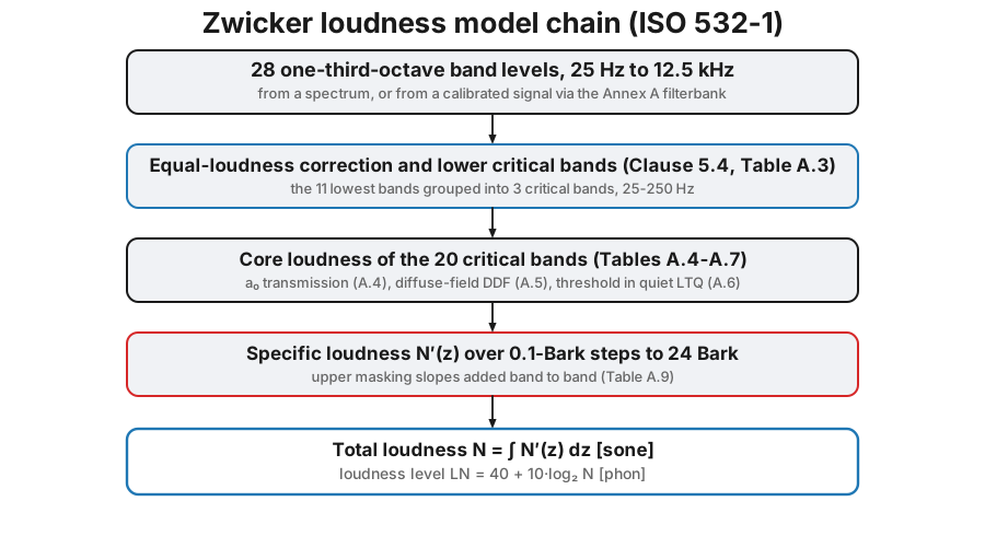
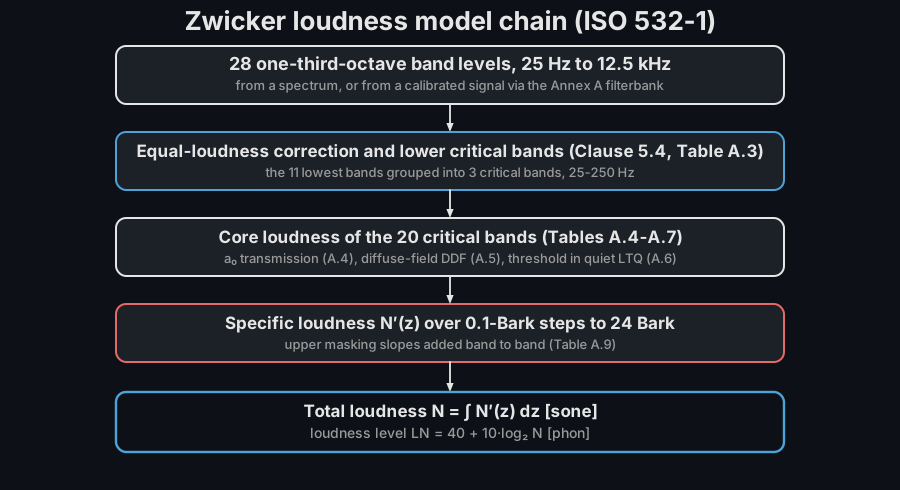
The animation below shows that integration at work: as the band level of a 1 kHz narrowband sound steps up, the specific-loudness pattern N’(z) grows along the Bark axis and the area under it is the total loudness in sones.

The specific-loudness pattern of a 1 kHz narrowband sound builds along the Bark axis as the band level steps from 45 to 85 dB, and the area under the pattern integrates to the total loudness in sones.

Download the animation (WebM)

The specific-loudness pattern of a 1 kHz narrowband sound builds along the Bark axis as the band level steps from 45 to 85 dB, and the area under the pattern integrates to the total loudness in sones.

Download the animation (WebM)

import numpy as np
from phonometry import psychoacoustics

# A raw recording plus its calibration so the guide runs standalone
fs = 48000
x = 0.2 * np.sin(2 * np.pi * 1000 * np.arange(fs) / fs)   # any recording (digital units)
sens = 1.0                                                # calibration_factor to pascals
levels_28 = np.full(28, 60.0)                             # 28 one-third-octave band levels (dB)

# From a raw recording: calibration_factor scales digital units to Pa
res = psychoacoustics.loudness_zwicker(x, fs, field="free", calibration_factor=sens)
print(f"N = {res.loudness:.1f} sone  ({res.loudness_level:.0f} phon)")   # 13.1 sone (77 phon)

# Time-varying signals: percentile loudness N5 is the reporting standard
res = psychoacoustics.loudness_zwicker(x, fs)          # stationary=False (default)
print(f"{res.n5:.1f} {res.n10:.1f} {res.loudness:.1f}")   # 13.1 13.1 13.1 — N5, N10, Nmax

# From 28 one-third-octave band levels (25 Hz .. 12.5 kHz)
res = psychoacoustics.loudness_zwicker_from_spectrum(levels_28, field="diffuse")

res.plot()   # N'(z) over the Bark scale — the specific-loudness pattern (needs matplotlib)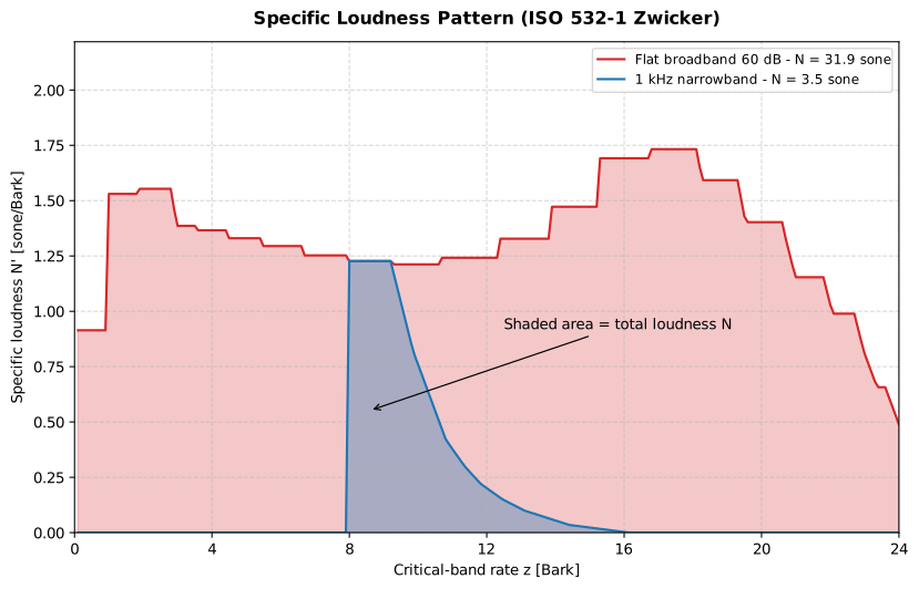

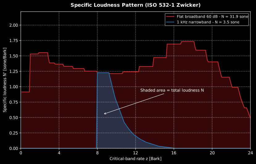
Same band level, very different loudness: energy spread over many critical bands (red) sums to far more sones than the same level concentrated in one band (blue). The area under N’(z) is the total loudness.

Show the code for this figure

import matplotlib.pyplot as plt
import numpy as np
from phonometry import psychoacoustics

levels_28 = np.full(28, 60.0)                             # 28 one-third-octave band levels (dB)
# From 28 one-third-octave band levels (25 Hz .. 12.5 kHz)
res = psychoacoustics.loudness_zwicker_from_spectrum(levels_28, field="diffuse")

# One line — the specific-loudness pattern N'(z) straight from the result:
res.plot()
plt.show()

# Or reproduce the figure by hand — two patterns of equal band level (60 dB),
# energy spread over many critical bands vs concentrated in the 1 kHz band:
narrow = psychoacoustics.loudness_zwicker_from_spectrum(np.r_[np.full(16, -60.0), 60.0, np.full(11, -60.0)])
broad = psychoacoustics.loudness_zwicker_from_spectrum(np.full(28, 60.0))
z = np.arange(1, narrow.specific.size + 1) * 0.1          # Bark axis
fig, ax = plt.subplots()
for r, color, label in [
    (broad, "#ff7f0e", f"Broadband  N = {broad.loudness:.1f} sone"),
    (narrow, "#1f77b4", f"1 kHz narrowband  N = {narrow.loudness:.1f} sone"),
]:
    ax.fill_between(z, r.specific, color=color, alpha=0.3)
    ax.plot(z, r.specific, color=color, label=label)
ax.set_xlabel("Critical-band rate z [Bark]")
ax.set_ylabel("Specific loudness N' [sone/Bark]")
ax.legend()
plt.show()

The implementation is a clean-room port of the standard’s normative reference program (Annex A.4): all twelve data tables are digit-exact and the full Annex B validation set runs in CI: the stationary test case reproduces the published value to every printed digit, and the tone-pulse N(t) traces stay inside the standard’s per-sample 5 % tolerance band.

loudness_zwicker() parameters

Parameter	Type	Units	Range / default	Notes
x	1D array	Pa (after calibration)	≥ 8 ms at 48 kHz	Resampled internally to 48 kHz if needed
fs	int	Hz	> 0
field	str	—	'free' (default) / 'diffuse'	Sound-field correction (Table A.5)
stationary	bool	—	default False	True: single N from the averaged spectrum
calibration_factor	float	Pa per digital unit	default 1.0	From sensitivity()

Returns a ZwickerLoudness dataclass: loudness (N, sones), loudness_level (phon), specific (N′(z), 240 bins of 0.1 Bark), and for time-varying runs n5, n10, time, loudness_vs_time (500 Hz trace).

ISO 532-1 report (.report())

ZwickerLoudness.report(path) renders a one-page PDF fiche laid out like an accredited loudness report: a standard-basis line, an optional metadata header block, a compact metrics table (total loudness N, loudness level L_N, and the N₅/N₁₀ percentiles for a time-varying result) beside the specific-loudness pattern N′(z) (the result’s own .plot()), the boxed N = X sone (LN = Y phon) single number, an optional verdict row and a footer with the fixed disclaimer. It uses the same ReportMetadata container and rendering engine as the ISO 717 insulation fiche; a supplied requirement is read as the maximum permitted loudness in sone (a lower loudness passes). Rendering needs reportlab (pip install phonometry[report]); only engine="reportlab" is supported. The fiche renders in English by default; pass language="es" for a Spanish fiche (translated fixed strings and a comma decimal separator), e.g. res.report("loudness_fiche_es.pdf", language="es").

from phonometry import psychoacoustics, ReportMetadata

res = psychoacoustics.loudness_zwicker_from_spectrum(levels_28, field="free")
res.report(
    "loudness_fiche.pdf",
    metadata=ReportMetadata(
        specimen="Household appliance, steady operating noise",
        measurement_standard="ISO 532-1 method 1",
        laboratory="Phonometry Reference Laboratory",
        requirement=12.0,             # maximum permitted loudness (sone)
    ),
)                                     # N (sone) and LN (phon)

The example fiche is regenerated with make reports and kept rendered in the repository; click the preview to open the PDF.

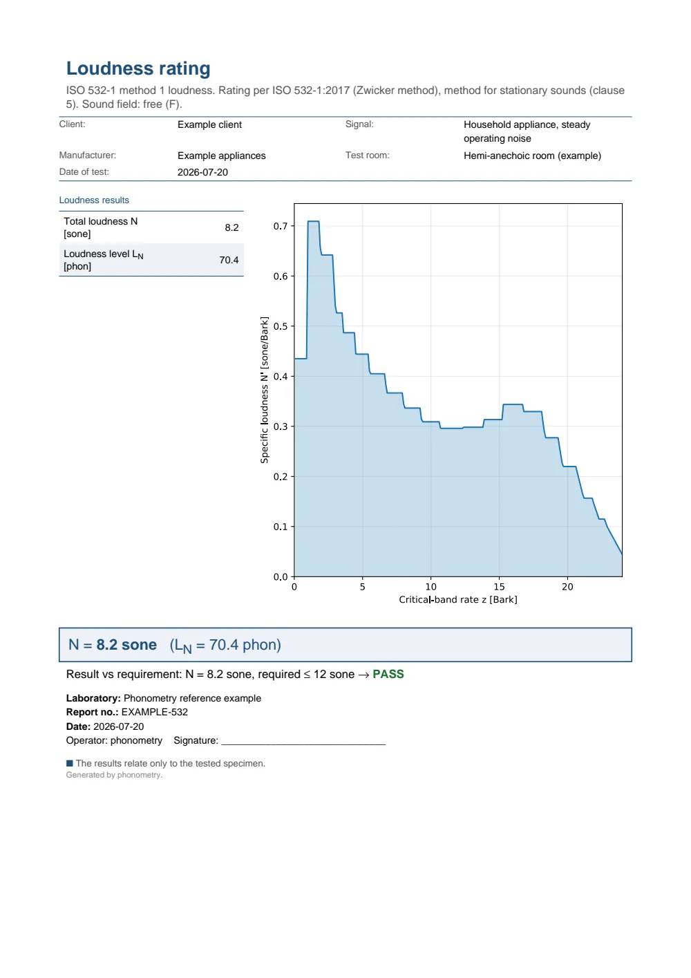
One-page loudness fiche: a metadata header, a metrics table with total loudness N and loudness level LN, the specific-loudness pattern over the critical-band rate, the boxed N = 8.2 sone (LN = 70.4 phon) single-number result and a PASS verdict against a 12 sone limit.

Download the report (PDF)

Zwicker loudness fiche (ZwickerLoudness.report), N in sone with LN in phon.

Loudness level of pure tones (ISO 226:2023)

The normal equal-loudness-level contours relate the SPL of a pure tone to its perceived loudness level in phons (the SPL of an equally loud 1 kHz tone). equal_loudness_contour(phon) evaluates ISO 226:2023 Formula (1) at the 29 preferred third-octave frequencies of Table 1, loudness_level(spl, frequency) is the exact inverse (Formula 2), and hearing_threshold() returns the threshold-of-hearing column. equal_loudness_contours(phons) bundles a whole family of contours with the threshold into a plottable EqualLoudnessContours result:

from phonometry import psychoacoustics

freqs, spl = psychoacoustics.equal_loudness_contour(40.0)   # the classic 40-phon contour
phon = psychoacoustics.loudness_level(73.0, 63.0)           # 73 dB @ 63 Hz -> 40 phon

# The whole family (20-90 phon by default) plus the hearing threshold:
res = psychoacoustics.equal_loudness_contours()
res.plot()   # the iconic ISO 226 chart (needs matplotlib)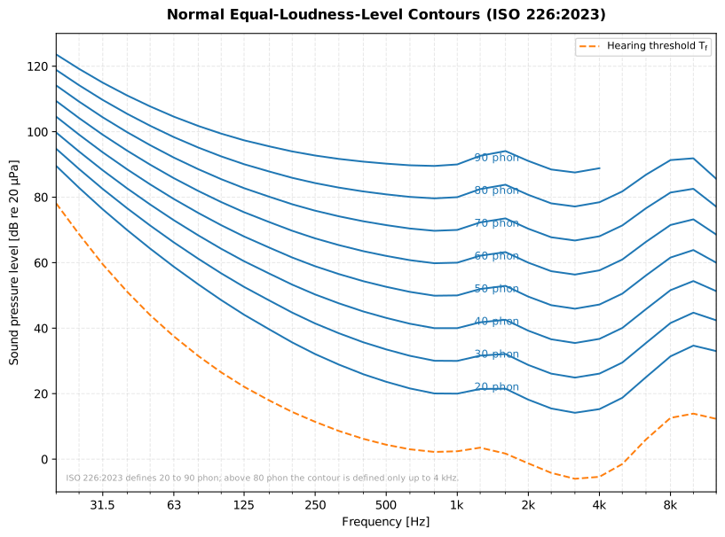

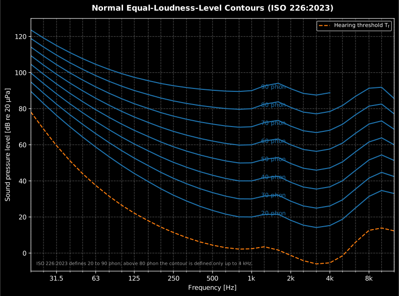
ISO 226:2023 defines the contours from 20 to 90 phon; above 80 phon the formula is valid only up to 4 kHz, so the 90 phon contour stops there and no higher contours are defined.

Show the code for this figure

import matplotlib.pyplot as plt
from phonometry import psychoacoustics

# One line — the contour family straight from the result:
res = psychoacoustics.equal_loudness_contours()
res.plot()
plt.show()

# Or reproduce the figure by hand — ISO 226:2023 Formula (1) at the 29
# preferred frequencies of Table 1, one contour per loudness level:
fig, ax = plt.subplots()
for phon in [20, 40, 60, 80, 90]:
    freqs, spl = psychoacoustics.equal_loudness_contour(float(phon))
    ax.semilogx(freqs, spl, color="C0")
    ax.annotate(f"{phon} phon", xy=(1000, phon + 1), fontsize=9)
ft, tf = psychoacoustics.hearing_threshold()
ax.semilogx(ft, tf, "--", color="C1", label="Hearing threshold $T_f$")
ax.set(xlabel="Frequency [Hz]", ylabel="Sound pressure level [dB re 20 µPa]")
ax.grid(True, which="both", alpha=0.3)
ax.legend()
plt.show()

Validity per clause 4.1: 20-90 phon (80 phon above 4 kHz); the implementation is verified against the Annex B tables in CI. Note this is the loudness of pure tones; the loudness of arbitrary signals in sones is what the ISO 532 models on this page compute.

Advanced loudness models

ISO 532-1 above is one of the three loudness model families phonometry ships (four methods in the table below). This section adds the Moore-Glasberg loudness of ISO 532-2/532-3 and the Sottek Hearing Model loudness of ECMA-418-2:2025, whose shared auditory front-end also powers the tonality and roughness metrics of Sound Quality Metrics.

Choosing a loudness model

Model	Standard	Stationary / time-varying	Output	When to use
Zwicker	ISO 532-1:2017	both	sone	Reference method; one-third-octave input; fast and widely cited
Moore-Glasberg	ISO 532-2:2017	stationary	sone	roex excitation pattern; better for tones and explicit binaural summation
Moore-Glasberg-Schlittenlacher	ISO 532-3:2023	time-varying	sone (STL/LTL)	Time-varying loudness with short-/long-term traces and the peak N_max
Sottek (Hearing Model)	ECMA-418-2:2025	time-varying	sone_HMS	Shares one auditory front-end with the ECMA tonality and roughness metrics

All four methods are anchored so a 1 kHz tone at 40 dB SPL is ≈ 1 sone; the values are not interchangeable digit-for-digit because the models differ in their auditory filters and their loudness summation.

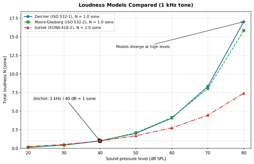
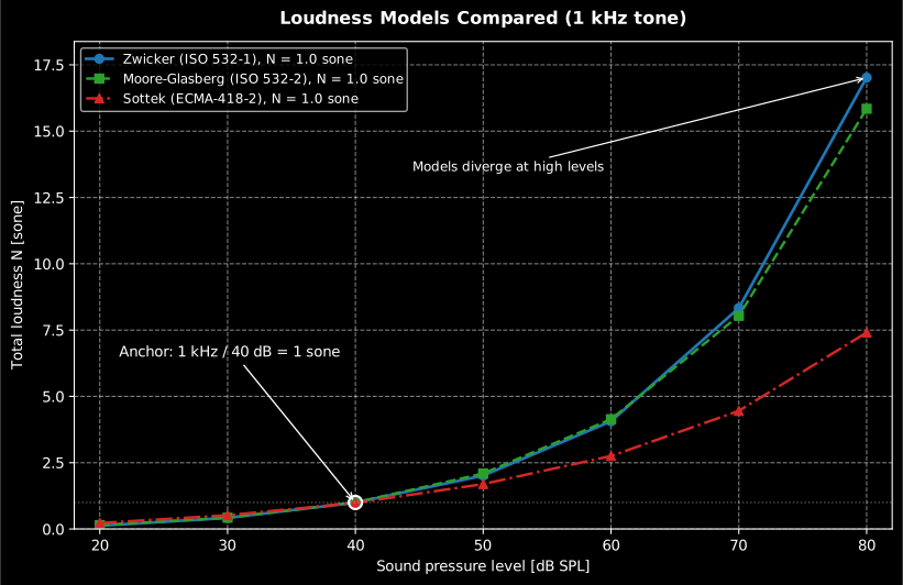
The three models agree at the 1 sone / 40 dB anchor and diverge with level: Zwicker doubles the sone value every +10 phon, while the Sottek model grows more slowly (about 1.65× per 10 dB), an intrinsic difference between the auditory summations, not a calibration error.

Show the code for this figure

import matplotlib.pyplot as plt
import numpy as np
from phonometry import psychoacoustics

# 1 kHz tone, 20..80 dB SPL: all three models pass through 1 sone at 40 dB
fs = 48000
t = np.arange(fs) / fs
levels = np.arange(20.0, 81.0, 10.0)
zw, mg, ec = [], [], []
for spl in levels:
    x = np.sqrt(2) * 2e-5 * 10 ** (spl / 20) * np.sin(2 * np.pi * 1000 * t)
    zw.append(psychoacoustics.loudness_zwicker(x, fs, stationary=True).loudness)
    mg.append(
        psychoacoustics.loudness_moore_glasberg_from_spectrum([(1000.0, float(spl))]).loudness
    )
    ec.append(psychoacoustics.loudness_ecma(x, fs).loudness)

fig, ax = plt.subplots()
ax.plot(levels, zw, "o-", label="Zwicker (ISO 532-1)")
ax.plot(levels, mg, "s--", label="Moore-Glasberg (ISO 532-2)")
ax.plot(levels, ec, "^-.", label="Sottek (ECMA-418-2)")
ax.plot(40.0, 1.0, "o", color="k", markerfacecolor="none", markersize=10)   # the shared anchor
ax.set(xlabel="Sound pressure level [dB SPL]", ylabel="Total loudness N [sone]")
ax.legend()
plt.show()

Moore-Glasberg loudness (ISO 532-2)

Where Zwicker uses fixed critical bands on the Bark scale, Moore-Glasberg builds an excitation pattern with level-dependent rounded-exponential (roex) auditory filters on the ERB-number (“Cam”) scale, then applies a compressive excitation → specific-loudness transform with C = 0.0617 sone/Cam (ISO 532-2:2017, Formula 7) and a binaural-inhibition stage. It reproduces the tone and broadband cases of Annex B to a percent or two and, unlike ISO 532-1, models binaural summation explicitly.

import numpy as np
from phonometry import psychoacoustics

# The definitional anchor: one 1 kHz sinusoidal component at 40 dB SPL,
# free field, binaural -> 1 sone / 40 phon by construction of the sone.
res = psychoacoustics.loudness_moore_glasberg_from_spectrum([(1000.0, 40.0)], field="free")
print(f"N = {res.loudness:.3f} sone  ({res.loudness_level:.1f} phon)")   # 1.000 sone (40.0 phon)

# From a calibrated recording: the narrowband (FFT) line spectrum is formed
# (power-preserving normalization) and fed to the exact sinusoidal-component
# method (ISO 532-2 clauses 5.2/5.4).
fs = 48000
x = np.sqrt(2) * 2e-5 * 10 ** (40 / 20) * np.sin(2 * np.pi * 1000 * np.arange(fs) / fs)
res = psychoacoustics.loudness_moore_glasberg(x, fs, field="free", presentation="binaural")

res.plot()   # specific loudness N'(i) over the ERB-number (Cam) scale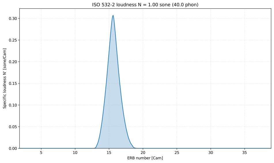

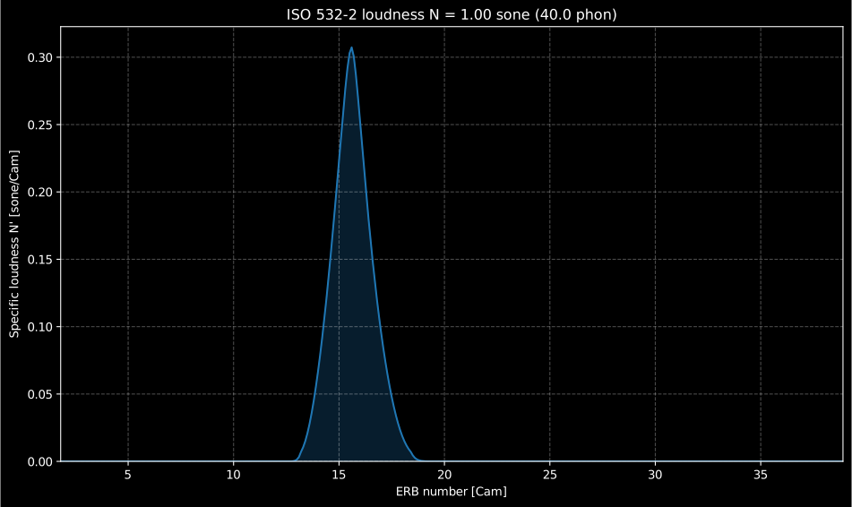
The ISO 532-2 pattern of the definitional 1 sone anchor. The peak is not a spectral line but the excitation the roex filters produce around the tone, so its width is the auditory filter, not the analysis resolution.

Show the code for this figure

import matplotlib.pyplot as plt
import numpy as np
from phonometry import psychoacoustics

# From a calibrated recording: the narrowband (FFT) line spectrum is formed
# (power-preserving normalization) and fed to the exact sinusoidal-component
# method (ISO 532-2 clauses 5.2/5.4).
fs = 48000
x = np.sqrt(2) * 2e-5 * 10 ** (40 / 20) * np.sin(2 * np.pi * 1000 * np.arange(fs) / fs)
res = psychoacoustics.loudness_moore_glasberg(x, fs, field="free", presentation="binaural")

# One line — the specific-loudness pattern N'(i) straight from the result:
res.plot()
plt.show()

# Or draw it by hand from the ERB-number grid the result already carries:
fig, ax = plt.subplots()
ax.fill_between(res.erb_number, res.specific, alpha=0.3)
ax.plot(res.erb_number, res.specific)
ax.set_xlabel("ERB number [Cam]")
ax.set_ylabel("Specific loudness N' [sone/Cam]")
plt.show()

loudness_moore_glasberg() parameters

Parameter	Type	Units	Range / default	Notes
x	1D array	Pa	non-empty	Calibrated pressure signal (signal wrapper)
components	list of (f, L)	Hz, dB SPL	—	_from_spectrum: discrete sinusoidal components
band_levels	29-vector	dB SPL	25 Hz .. 16 kHz	_from_third_octave input (IEC 61260-1 bands)
fs	int	Hz	> 0	Signal wrapper only
field	str	—	'free' (default) / 'diffuse' / 'eardrum'	Outer-ear transfer
presentation	str	—	'binaural' (default) / 'diotic' / 'monaural'	Binaural summation

Returns a MooreGlasbergLoudness: loudness (N, sone), loudness_level (phon), specific (N′(i), 372 bins of 0.1 Cam), erb_number, centre_frequencies, field, presentation.

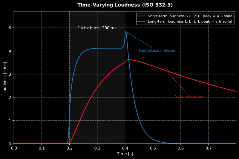
Time-varying loudness (ISO 532-3)

ISO 532-3 wraps the same excitation / specific-loudness model in a running multi-resolution spectral analysis (six parallel FFTs, updated every 1 ms) and two cascaded temporal integrators: the fast short-term loudness S′(t) and the slower long-term loudness S″(t). The peak long-term loudness N_max predicts the loudness of sounds up to about 5 s.

import numpy as np
from phonometry import psychoacoustics

fs = 32000
t = np.arange(int(1.3 * fs)) / fs
x = np.sqrt(2) * 2e-5 * 10 ** (40 / 20) * np.sin(2 * np.pi * 1000 * t)

res = psychoacoustics.loudness_moore_glasberg_time(x, fs, field="free")
print(f"N_max = {res.n_max:.3f} sone  ({res.loudness_level_max:.0f} phon)")   # 1.000 sone (40 phon)
print(f"long-term loudness exceeded 5% of the time: {res.percentiles[5.0]:.3f} sone")   # 0.999 sone

res.plot()   # short-term S'(t) and long-term S''(t) loudness vs time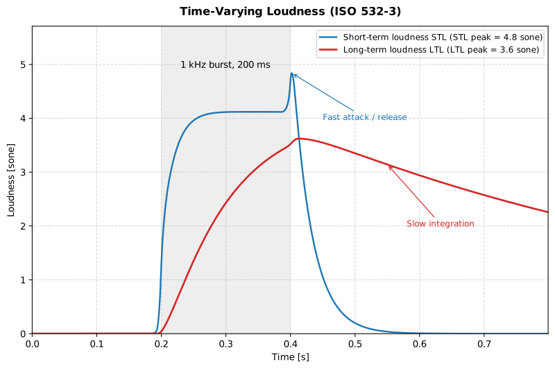

Show the code for this figure

import matplotlib.pyplot as plt
import numpy as np
from phonometry import psychoacoustics

fs = 32000
t = np.arange(int(1.3 * fs)) / fs
x = np.sqrt(2) * 2e-5 * 10 ** (40 / 20) * np.sin(2 * np.pi * 1000 * t)
res = psychoacoustics.loudness_moore_glasberg_time(x, fs, field="free")

# The result carries both traces on a 1 ms time axis:
res.plot()
plt.show()

# Or plot them directly to see the fast STL vs the slow LTL:
fig, ax = plt.subplots()
ax.plot(res.time, res.short_term_loudness, label="Short-term S'(t)")
ax.plot(res.time, res.long_term_loudness, label="Long-term S''(t)")
ax.set_xlabel("Time [s]")
ax.set_ylabel("Loudness [sone]")
ax.legend()
plt.show()

loudness_moore_glasberg_time() parameters

Parameter	Type	Units	Range / default	Notes
signal	1D or (n, 2) array	Pa	non-empty	Mono = diotic; two columns = left/right ears
fs	int	Hz	> 0
field	str	—	'free' (default) / 'diffuse' / 'eardrum'	Outer-ear transfer
presentation	str	—	'binaural' (default) / 'diotic' / 'monaural'	Binaural summation
percentiles	sequence	percent	default (1, 5, 10, 50, 90, 95)	Exceeded long-term loudness levels

Returns a MooreGlasbergTimeVaryingLoudness: time (1 ms grid), short_term_loudness / long_term_loudness (sone), their _level in phon, n_max, loudness_level_max, a percentiles dict, field, presentation.

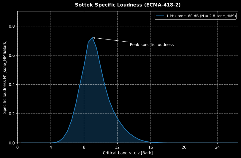
Sottek Hearing Model loudness (ECMA-418-2)

ECMA-418-2:2025 specifies a single auditory front-end (outer/middle-ear filtering, a 53-band gammatone-like filter bank on the Bark_HMS scale with z = 0.5 .. 26.5, half-wave rectification, block RMS and a compressive nonlinearity, Formula 23) that is shared by its loudness, tonality and roughness metrics. The loudness N is reported in sone_HMS, and the same 1 kHz/40 dB anchor calibrates the front-end (our clean-room value 0.984, with the full Clause 6.2.3 band averaging; the residual’s origin is documented in the module docstring).

import numpy as np
from phonometry import psychoacoustics

fs = 48000
t = np.arange(int(1.2 * fs)) / fs
x = np.sqrt(2) * 2e-5 * 10 ** (40 / 20) * np.sin(2 * np.pi * 1000 * t)

res = psychoacoustics.loudness_ecma(x, fs, field="free")
print(f"N = {res.loudness:.3f} sone_HMS")   # 0.984 sone_HMS
print(res.specific_loudness.shape)          # (53,) average specific loudness N'(z)

res.plot()   # average specific loudness N'(z) + time-dependent N(l) at 187.5 Hz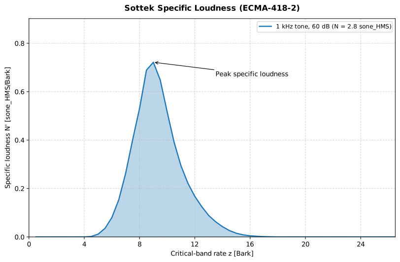

Show the code for this figure

import matplotlib.pyplot as plt
import numpy as np
from phonometry import psychoacoustics

fs = 48000
t = np.arange(int(1.2 * fs)) / fs
x = np.sqrt(2) * 2e-5 * 10 ** (40 / 20) * np.sin(2 * np.pi * 1000 * t)
res = psychoacoustics.loudness_ecma(x, fs, field="free")

# The result carries the average specific loudness over the 53 Bark_HMS bands:
res.plot()
plt.show()

# Or draw N'(z) by hand against the critical-band-rate scale:
fig, ax = plt.subplots()
ax.fill_between(res.bark, res.specific_loudness, alpha=0.3)
ax.plot(res.bark, res.specific_loudness)
ax.set_xlabel("Critical-band rate z [Bark_HMS]")
ax.set_ylabel("Specific loudness N' [sone_HMS/Bark_HMS]")
plt.show()

loudness_ecma() parameters

Parameter	Type	Units	Range / default	Notes
signal_in	1D array	Pa	non-empty	Calibrated pressure signal
fs	float	Hz	> 0	Resampled to 48 kHz internally if needed (Clause 5.1.1)
field	str	—	'free' (default) / 'diffuse'	Outer/middle-ear filter (Clause 5.1.3)

Returns an EcmaLoudness: loudness (N, sone_HMS), specific_loudness (N′(z), 53 bands), bark, centre_frequencies, time, loudness_vs_time (N(l) at 187.5 Hz), field.

What this guide covers

Covered. ISO 532-1:2017 (Zwicker method): the stationary method of clause 5 and the time-varying method of clause 6, ported from the normative Annex A.4 reference program and validated against Annex B, with the n5/n10 percentiles, via loudness_zwicker() and loudness_zwicker_from_spectrum(). ISO 532-2:2017 (Moore-Glasberg): the roex excitation pattern of clause 7 and the binaural inhibition of clause 8, via loudness_moore_glasberg() and its _from_spectrum/_from_third_octave variants. ISO 532-3:2023 (Moore-Glasberg-Schlittenlacher): the short-term loudness of clause 7.8, the long-term loudness of clause 7.9 and its peak N_max, via loudness_moore_glasberg_time(). ECMA-418-2:2025 (Sottek Hearing Model): the loudness assembly of Clause 8, via loudness_ecma(). ISO 226:2023: Formula (1), Formula (2) and the Table 1 contour parameters, via equal_loudness_contour(), loudness_level(), hearing_threshold() and equal_loudness_contours().

Not covered. ECMA-418-2’s binaural combination (Formula 118, Clause 8.1.5) is not implemented: loudness_ecma() is monaural, so analyse each ear channel separately. ISO 532-3 Clause 5 prescribes resampling the input to 32 kHz before the running FFT analysis. This implementation processes at the native sampling rate instead, a documented deviation that stays inside the standard’s expanded uncertainty. Resample to 32 kHz first if strict clause-by-clause conformance matters.

See also

• Sound Quality Metrics: sharpness, tonality and roughness, the other half of the sound-quality story.
• Psychoacoustic annoyance and fluctuation strength: the Zwicker and Fastl model that consumes the percentile loudness N5.
• Theory: the equations behind the loudness models.
• API reference: psychoacoustics.loudness_zwicker, psychoacoustics.loudness_moore_glasberg and psychoacoustics.loudness_contours.

Quick answers

What is the difference between loudness in sones and loudness level in phons?

Loudness N in sones (ISO 532-1) is a ratio scale of perceived loudness: 4 sones is twice as loud as 2 sones, and by definition a 1 kHz tone at 40 dB SPL is 1 sone. Loudness level in phons (ISO 226) is the SPL of an equally loud 1 kHz pure tone, and every +10 phon doubles the sone value.

Which loudness model should I choose: Zwicker, Moore-Glasberg or Sottek?

The Zwicker method (ISO 532-1:2017) is the reference: stationary and time-varying, one-third-octave input, fast and widely cited. Moore-Glasberg (ISO 532-2:2017) is stationary, builds roex excitation patterns and models binaural summation explicitly; ISO 532-3:2023 adds time-varying short- and long-term loudness with the peak N_max. The Sottek model (ECMA-418-2:2025) reports sone_HMS and shares its auditory front-end with the ECMA tonality and roughness metrics.

Over what range are the ISO 226:2023 equal-loudness contours valid?

ISO 226:2023 clause 4.1 defines the normal equal-loudness-level contours from 20 to 90 phon, evaluated at the 29 preferred third-octave frequencies of Table 1; above 80 phon the formula is valid only up to 4 kHz, so the 90 phon contour stops there and no higher contours are defined. The contours describe pure tones, not arbitrary signals.

References

• Ecma International. (2025). Psychoacoustic metrics for ITT equipment — Part 2 (methods for describing human perception based on the Sottek Hearing Model) (ECMA-418-2, 4th ed.). The Sottek Hearing Model loudness (sone_HMS).
• Fastl, H., & Zwicker, E. (2007). Psychoacoustics: Facts and models (3rd ed.). Springer. https://doi.org/10.1007/978-3-540-68888-4The critical-band and masking psychoacoustics behind the Zwicker model and the loudness sensation the newer models refine.
• Fletcher, H., & Munson, W. A. (1933). Loudness, its definition, measurement and calculation. The Journal of the Acoustical Society of America, 5(2), 82-108. https://doi.org/10.1121/1.1915637The original equal-loudness measurements behind the loudness-level concept of the pure-tone section.
• International Organization for Standardization. (2017). Acoustics — Methods for calculating loudness — Part 1: Zwicker method (ISO 532-1:2017). Stationary and time-varying loudness in sones from the normative Annex A.4 reference program, with the N5/N10 percentile loudness, validated against the Annex B set.
• International Organization for Standardization. (2017). Acoustics — Methods for calculating loudness — Part 2: Moore-Glasberg method (ISO 532-2:2017). Stationary loudness from roex excitation patterns on the ERB-number scale, with explicit binaural summation.
• International Organization for Standardization. (2023). Acoustics — Methods for calculating loudness — Part 3: Moore-Glasberg-Schlittenlacher method (ISO 532-3:2023). Time-varying short-term and long-term loudness and the peak N_max.
• International Organization for Standardization. (2023). Acoustics — Normal equal-loudness-level contours (ISO 226:2023). The contour model and Table 1 parameters behind the pure-tone loudness levels: the contours (Formula 1), the loudness level of pure tones (Formula 2) and the hearing threshold.