Room to Room: Partition, Receiving Room, Criterion

Standards: ANSI/ASA S12.2Key references: Norton & Karczub 2003 Bies et al. 2017 Kuttruff 2016

A machine runs in one room, a wall separates that room from an occupied one, and someone wants to know what the occupant hears. It is a short chain of four links — the reverberant level the machine builds up on the source side, the transmission loss of the wall, the absorption of the receiving room, and the criterion the result is laid against — and the joint between the second and the third is where the arithmetic surprises people: the noise reduction is not the transmission loss of the wall.

noise_control.room_to_room is that joint, and this page walks Norton & Karczub’s worked problems through it end to end. The reference throughout is Norton, M. P. & Karczub, D. G., Fundamentals of Noise and Vibration Analysis for Engineers (2nd ed., Cambridge University Press 2003), Chapter 4: §4.6 for the sound power models, §4.9 for the room-to-room balance and §4.10 for the enclosure. Its problems 4.16, 4.18 and 4.21 carry printed octave-band answers, and all three are pinned in the conformance report.

Here is the whole page in one drawing — Norton’s problem 4.18 in section, with every symbol of the balance sitting where it physically belongs.

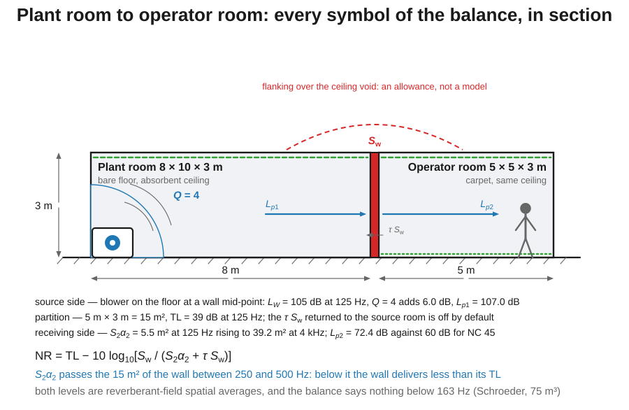
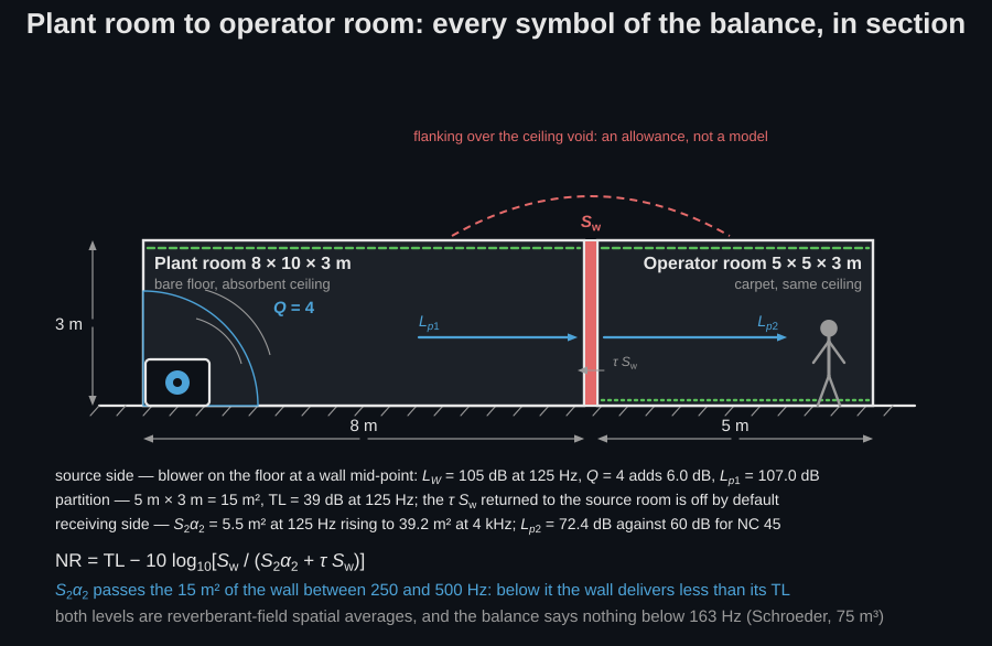
Where the partition itself comes from is a different question, answered by Panel sound insulation (mass law, coincidence, double leaves, the plateau method) or by measurement. This page takes the transmission loss as given, exactly as a hand calculation does.

1. What the balance says

Norton’s §4.9 balances the steady-state power in the receiving room: what crosses the partition equals what the room absorbs plus what leaks back through the partition. Replacing intensities with mean-square pressures and taking logarithms gives Equation (4.101),

NR = TL - 10 lo g_{10} [\frac{S _{w}}{S _{2} α _{2} + τ S _{w}}],

with $NR = L_{p 1} - L_{p 2}$ the noise reduction between the two reverberant fields, $TL = 10 lo g_{10} (1/ τ)$ the transmission loss of the partition — the name Norton & Karczub and the North American literature use for the quantity ISO 10140-2 measures and ISO 717-1 rates as the sound reduction index $R$ ; they are the same number, and its single-number rating is the $R_{w}$ used below, so the $R$ and $R_{w}$ of a laboratory test report drop straight into this equation (see Insulation ratings (ISO 717)) — $S_{w}$ the area of the partition and $S_{2} α_{2}$ the equivalent absorption area of the receiving room.

Read the logarithm and the whole page follows. A large partition into a hard room delivers less than its transmission loss: a lot of area radiating into a room with nothing to soak it up. A small partition into a well-absorbing room delivers more. The two rooms and the wall are not separable, which is why quoting a wall’s $R_{w}$ and stopping is not an answer.

The $τ S_{w}$ term is the power the partition itself passes back into the source room. At any realistic transmission loss it is worth a few hundredths of a decibel, so it is off by default and include_partition_transmission=True switches it on.

What a measurement of the same pair reports

The $NR$ of this equation is the raw level difference $D$ that a field measurement of the two rooms returns. Measurement standards do not report $D$ raw, and for the reason this section has just given: $D$ depends on the receiving room. They normalise it, either to a reference reverberation time, $D_{n T} = D + 10 lo g_{10} (T / T_{0})$ with $T_{0} = 0.5$ s — the quantity most residential regulations are written in — or to a reference absorption area of 10 m², $D_{n} = D - 10 lo g_{10} (A /10)$ . The wall’s own quantity is $R$ , and the field version of it, $R^{'} = D + 10 lo g_{10} (S / A)$ , includes flanking and is therefore always below the laboratory $R$ this calculation assumes.

The consequence is worth stating flatly: a computed $NR$ and a certified $D_{n T, w}$ for the same wall are different numbers by construction, and comparing them without renormalising is the commonest way to conclude that the model is wrong when it is not. The receiving-room reverberation time has to be measured in the same session, because it is what carries the normalisation. Field sound insulation has the source and microphone positions, the minimum separations and the background-noise correction; Laboratory sound insulation has where a declared $R$ comes from.

2. Three partitions, one receiving room

Norton’s problem 4.21 (printed pp. 586-587) is the comparison the equation was made for: two 13 mm gypsum wallboards with a 64 mm air gap, a 125 mm plastered brick wall and a double brick wall with a 50 mm cavity, all speaking into the same 8 m x 9 m x 3 m receiving room through the same 8 m x 3 m opening.

import numpy as np
from phonometry import (
    SourceRoom, equivalent_absorption_area, room_to_room_transmission,
)

bands = [125.0, 250.0, 500.0, 1000.0, 2000.0, 4000.0]

# Receiving room 8 x 9 x 3 m: walls 102 m2, floor and ceiling 72 m2 each.
receiving = equivalent_absorption_area([
    (102.0, [0.04, 0.04, 0.09, 0.15, 0.17, 0.23]),   # walls
    (72.0,  [0.02, 0.06, 0.14, 0.37, 0.60, 0.66]),   # floor
    (72.0,  [0.30, 0.20, 0.15, 0.05, 0.05, 0.05]),   # ceiling
])
print(np.round(receiving, 1))
# [27.1 22.8 30.1 45.5 64.1 74.6]   m2, band by band

partitions = {
    "Two 13 mm wallboards, 64 mm gap": [18, 27, 37, 45, 43, 39],
    "125 mm plastered brick":          [36, 36, 40, 46, 54, 57],
    "Double brick, 50 mm cavity":      [37, 41, 48, 60, 61, 61],
}
for name, tl in partitions.items():
    res = room_to_room_transmission(
        bands, tl, 8.0 * 3.0, receiving,
        source=SourceRoom(level=90.0), label=name,
    )
    print(f"{name:32s} {np.round(res.noise_reduction, 1)}")
# Two 13 mm wallboards, 64 mm gap  [18.5 26.8 38.  47.8 47.3 43.9]
# 125 mm plastered brick           [36.5 35.8 41.  48.8 58.3 61.9]
# Double brick, 50 mm cavity       [37.5 40.8 49.  62.8 65.3 65.9]

Those are Norton’s printed answers to the tenth of a decibel. Look at what the receiving room did to them. At 125 Hz the room absorbs 27.1 m² against a 24 m² partition, so every wall delivers half a decibel more than its transmission loss. At 250 Hz the ceiling has stopped absorbing and the floor has not started, the room is down to 22.8 m², and every wall now delivers 0.2 dB less. By 4 kHz the carpet and the walls together give 74.6 m² and the same brick wall is worth 4.9 dB more than its transmission loss. The same three walls, ranked the same way, but the numbers a specification would quote move by more than 5 dB depending on a room the wall never touches.

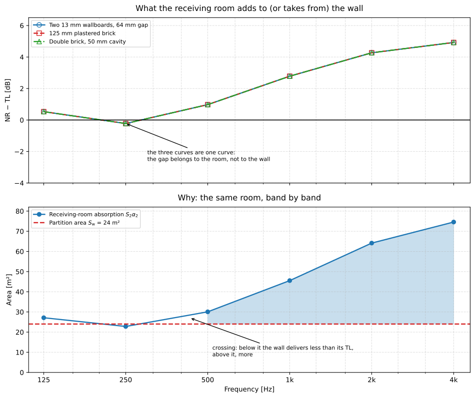
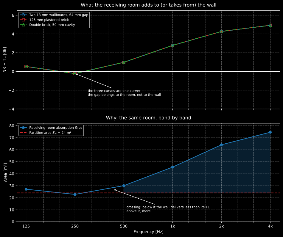
Two stacked octave-band panels from 125 Hz to 4 kHz. Above, the noise reduction minus the transmission loss for the three partitions: the three curves fall exactly on top of one another, starting at plus 0.5 dB at 125 Hz, dipping to minus 0.2 dB at 250 Hz and rising to plus 4.9 dB at 4 kHz. Below, the receiving room's equivalent absorption area rising from 27 square metres at 125 Hz through a dip to 23 at 250 Hz and on to 75 at 4 kHz, against the fixed 24 square metres of the partition drawn as a horizontal dashed line, with the region above the line shaded

Subtract each wall’s transmission loss from the noise reduction it delivers and the three partitions collapse onto one curve, because the difference, $- 10 lo g_{10} [S_{w} / (S_{2} α_{2})]$ , contains no property of the wall at all. It is the lower panel: the gap changes sign exactly where the receiving room’s absorption area crosses the 24 m² of the partition. Ranking three walls is safe; quoting the decibels one of them “gives” is not.

Show the code for this figure

import matplotlib.pyplot as plt

# `bands`, `receiving` and `partitions` as built above.

# One line per wall: the RoomToRoomResult draws both spectra, the criterion
# and the noise reduction against the transmission loss.
room_to_room_transmission(
    bands, partitions["125 mm plastered brick"], 8.0 * 3.0, receiving,
    source=SourceRoom(level=90.0),
).plot()
plt.show()

# By hand: the gap each wall shows, and the room behind it.
fig, (top, bottom) = plt.subplots(2, 1, sharex=True)
for name, tl in partitions.items():
    res = room_to_room_transmission(bands, tl, 8.0 * 3.0, receiving,
                                    source=SourceRoom(level=90.0))
    top.semilogx(bands, res.noise_reduction - np.asarray(tl, float),
                 "o-", label=name)
top.axhline(0.0)
bottom.semilogx(bands, receiving, "o-", label="Receiving-room absorption")
bottom.axhline(8.0 * 3.0, ls="--", label="Partition area")
bottom.set_xlabel("Frequency [Hz]")
plt.show()

3. The chain, end to end

Problem 4.18 (printed pp. 585-586) is the whole calculation, and it starts one step earlier: the source-room level is not given, only the blower’s free-field sound power level. Two decisions turn that into $L_{p 1}$ , and both are Norton’s.

The reverberant field is what drives the partition. The receiver of interest is the wall, not a point beside the machine, so the level that matters is $L_{p 1} = L_{W} + 10 lo g_{10} (4/ R_{1})$ . That is steady_state_spl with distance=None, the $r \to \infty$ limit of the same Bies Equation (6.43) the library has always used for a receiver at a distance.

The problem asks for a conservative estimate, and conservative has a meaning. The blower sits on the floor along the middle of a wall, in the intersection of two large flat surfaces, so $Q = 4$ . Norton’s §4.6 Table 4.5 lists three sound power models: a constant-power source radiates the same $Π_{0}$ wherever it stands, a constant-volume source is loaded by the nearby boundaries and radiates $Π_{0} Q$ , and a constant-pressure source, a theoretical floor, radiates $Π_{0} / Q$ . Real machines sit between the first two whenever they are closer to the boundary than a wavelength, and the constant-volume model is the upper bound. Here it is worth $10 lo g_{10} 4 = 6.02 dB$ , and without it the printed answers come out 6 dB low.

from phonometry import (
    DesignCriterion, SourceRoom, equivalent_absorption_area, mean_absorption,
    room_constant, room_to_room_transmission,
)

bands = [125.0, 250.0, 500.0, 1000.0, 2000.0, 4000.0]
ceiling = [0.07, 0.20, 0.40, 0.52, 0.60, 0.67]      # absorbent ceiling
walls = [0.03, 0.03, 0.03, 0.04, 0.05, 0.07]        # both rooms

# Plant room 8 x 10 x 3 m: bare floor, absorbent ceiling, 108 m2 of wall.
plant = [(80.0, [0.01, 0.01, 0.015, 0.02, 0.02, 0.02]),
         (80.0, ceiling), (108.0, walls)]

# Operator room 5 x 5 x 3 m: carpet, same ceiling and walls.
operator = [(25.0, [0.08, 0.24, 0.57, 0.69, 0.71, 0.73]),
            (25.0, ceiling), (60.0, walls)]

chain = room_to_room_transmission(
    bands,
    [39.0, 42.0, 50.0, 58.0, 63.0, 67.0],       # TL of the separating wall
    5.0 * 3.0,                                  # the wall is 5 m x 3 m
    equivalent_absorption_area(operator),
    source=SourceRoom(
        power_level=[105.0, 103.0, 98.0, 108.0, 107.0, 109.0],
        room_constant=room_constant(268.0, mean_absorption(plant)),
        directivity=4.0,                        # floor-wall intersection
        model="constant_volume",                # the conservative bound
    ),
    criterion=DesignCriterion(target=45.0),
    label="Plant room to operator room",
)

for row in chain.table():
    print(f"{row['label']:<28} "
          f"{[round(float(v), 1) for v in row['values']]}")

Two similarly named functions do two different jobs in that snippet, and swapping them is silent. $A = S α$ , equivalent_absorption_area, is the power the room removes per unit mean-square pressure, and it is what appears in the receiving-room balance of Equation (4.101). $R = S α / (1 - α)$ , room_constant, is the room constant of the steady-state relation, which also accounts for the energy that survives its first reflection and goes on feeding the reverberant field, and it is what $L_{p 1} = L_{W} + 10 lo g_{10} (4/ R)$ needs on the source side. The two coincide for a live room and diverge as $α$ grows — they differ by $10 lo g_{10} [1/ (1 - α)]$ , 0.5 dB at $α = 0.1$ and 3.0 dB at $α = 0.5$ — and using the absorption area where the room constant belongs biases the answer towards predicting too much noise reduction. equivalent_absorption_area also takes discrete objects and an air-absorption term, which is how furniture, people and, in a large room, the air itself enter the receiving side.

Source sound power level     [105.0, 103.0, 98.0, 108.0, 107.0, 109.0]
Source room level            [107.0, 101.7, 93.8, 102.4, 100.6, 101.9]
Partition transmission loss  [39.0, 42.0, 50.0, 58.0, 63.0, 67.0]
Receiving-room absorption    [5.5, 12.8, 26.1, 32.6, 35.8, 39.2]
Noise reduction              [34.7, 41.3, 52.4, 61.4, 66.8, 71.2]
Receiving room level         [72.4, 60.4, 41.4, 41.0, 33.9, 30.7]
NC 45                        [60.0, 54.0, 49.0, 46.0, 44.0, 43.0]
Required transmission loss   [51.4, 48.4, 42.4, 53.0, 52.9, 54.7]

Norton’s printed answer is 72.3 / 60.4 / 41.4 / 41.0 / 33.8 / 30.7 dB, which this reproduces to a tenth. Two rows are worth staring at. The noise reduction climbs from 34.7 dB to 71.2 dB while the transmission loss only climbs from 39 to 67, because the operator room’s absorption grows sevenfold across the range while the wall is fixed at 15 m²; the little room does half the work at high frequency and none at all at 125 Hz. And the required transmission loss row is not monotone: the wall needs 51.4 dB at 125 Hz where it has 39, and 42.4 dB at 500 Hz where it already has 50. A low-frequency problem, in a wall that is over-specified in the middle.

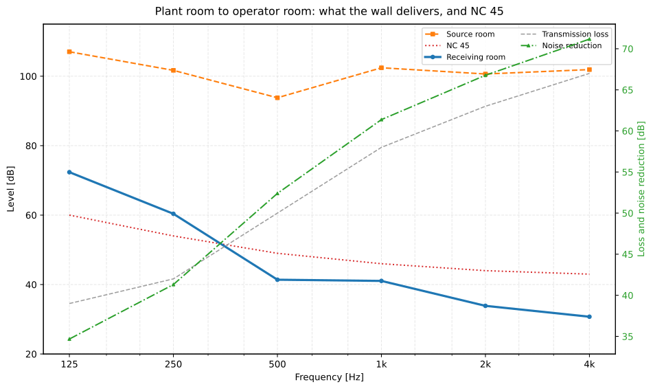
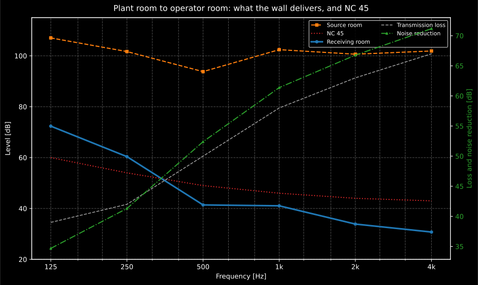
Octave-band chart of Norton's plant-room problem from 125 Hz to 4 kHz: the source-room level runs from 107 dB down to 94 dB at 500 Hz and back to 102 dB, the receiving-room level falls steadily from 72 dB to 31 dB and crosses the NC 45 curve between 250 and 500 Hz, and on the right axis the transmission loss of the wall rises from 39 to 67 dB while the noise reduction it delivers rises from 35 to 71 dB, crossing the transmission loss between 250 and 500 Hz

The chain of problem 4.18. The receiving-room spectrum crosses the NC 45 curve between 250 and 500 Hz, so the two low bands are the whole problem. The right axis is the point of Equation (4.101): the noise reduction the wall delivers starts 4 dB below its transmission loss and ends 4 dB above it, and the crossing is where the operator room’s absorption grows past the 15 m² of the wall.

Show the code for this figure

import matplotlib.pyplot as plt

# `chain` is the RoomToRoomResult built above.

# One line: both reverberant spectra, the criterion curve and the noise
# reduction against the transmission loss on the twin axis.
chain.plot()
plt.show()

# By hand, from the per-band fields the result carries:
fig, ax = plt.subplots()
ax.semilogx(chain.frequencies, chain.source_level, "s--", label="Source room")
ax.semilogx(chain.frequencies, chain.received_level, "o-", label="Receiving room")
ax.semilogx(chain.frequencies, chain.criterion_curve, ":", label="NC 45")
twin = ax.twinx()
twin.plot(chain.frequencies, chain.transmission_loss, "--", label="TL")
twin.plot(chain.frequencies, chain.noise_reduction, "-.", label="NR")
plt.show()

4. The verdict, and the number to specify

The result rates itself. .rating is the ANSI/ASA S12.2-2019 rating of the received spectrum, .criterion_curve is the design curve sampled at the analysis bands, .exceedance is the band-by-band excess and .meets_target is the plain verdict a design sheet writes down. .required_transmission_loss is Equation (4.101) solved for $TL$ , which is the number that goes into a specification.

print(chain.meets_target)                       # False
print(round(chain.rating.rating, 1))            # 61.7, governed by 125 Hz
print([round(float(v), 1) for v in chain.exceedance])
# [12.4, 6.4, -7.6, -5.0, -10.1, -12.3]

deficit = chain.required_transmission_loss - chain.transmission_loss
print([round(float(v), 1) for v in deficit])
# [12.4, 6.4, -7.6, -5.0, -10.1, -12.3]

The deficit and the exceedance are the same six numbers, which is the whole content of the chain: a decibel too much in the room is a decibel too little in the wall. Whether that low-frequency deficit is worth chasing with mass, a cavity or a second leaf is what Panel sound insulation is for.

The verdict is deliberately the band-by-band test, not the rating. A spectrum can rate NC-38 and still poke through the NC 45 curve in one band, because the standard’s two-step designation procedure and a design sheet’s “no band above the curve” are different questions.

5. An enclosure against a criterion

Problem 4.16 (printed pp. 584-585) asks the same question about an enclosure instead of a partition: a refrigeration compressor makes a reverberant level in its room, the technician needs that level down to an NC-45 curve, and the enclosure walls have to make up the difference. Norton derives the enclosure equation from the same power balance as §4.9 and gets Equation (4.115),

IL = TL - 10 lo g_{10} (S_{E} / R_{i}),

with $S_{E}$ the external radiating area and $R_{i}$ the room constant of the enclosure interior, machine surface included. Solved for the panels, $TL = IL + 10 lo g_{10} (S_{E} / R_{i})$ , which is enclosure_required_transmission_loss.

import numpy as np
from phonometry import enclosure_required_transmission_loss, mean_absorption

bands = [63.0, 125.0, 250.0, 500.0, 1000.0, 2000.0, 4000.0, 8000.0]
wool = [0.10, 0.20, 0.45, 0.65, 0.75, 0.80, 0.80, 0.80]   # 50 mm blanket
concrete = [0.01, 0.01, 0.01, 0.02, 0.02, 0.02, 0.03, 0.03]

lp1 = np.array([72.0, 79.0, 81.0, 84.0, 83.0, 81.0, 80.0, 75.0])   # unenclosed
nc45 = np.array([67.0, 60.0, 54.0, 49.0, 46.0, 44.0, 43.0, 41.0])  # target

# Enclosure 2.5 x 3.5 x 2.5 m on the concrete floor: the walls and roof
# radiate (38.75 m2) and their inner faces carry the lining. The rest of the
# interior is the uncovered floor plus the five exposed faces of the
# 1.5 x 2.5 x 1.5 m machine, both with the absorption of concrete.
radiating = 2 * (2.5 * 2.5) + 2 * (3.5 * 2.5) + 2.5 * 3.5
machine = 2 * (1.5 * 1.5) + 2 * (2.5 * 1.5) + 1.5 * 2.5
bare_floor = 2.5 * 3.5 - 1.5 * 2.5

required = enclosure_required_transmission_loss(
    lp1 - nc45,
    radiating,
    radiating + bare_floor + machine,
    mean_absorption([(radiating, wool), (bare_floor + machine, concrete)]),
    frequencies=bands,
    model="norton",
)
print(np.round(required.panel_transmission_loss, 1))
# [14.5 25.3 28.9 34.4 35.2 34.7 34.6 31.6]

Norton’s printed answer is 14.4 / 25.2 / 28.9 / 34.4 / 35.2 / 34.7 / 34.7 / 31.6 dB, matched to 0.11 dB, which is the resolution of his own one-decimal rounding. The shape is the useful part: the requirement peaks at 1 kHz and falls away at both ends, because at 63 Hz the mineral wool absorbs almost nothing and the level to lose is only 5 dB, while at 8 kHz the compressor has quietened down. A panel chosen for its 500 Hz to 2 kHz figure is the right panel here.

enclosure_required_transmission_loss returns an EnclosureResult, so required.plot() draws that shape and its two causes in one line:

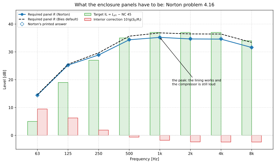
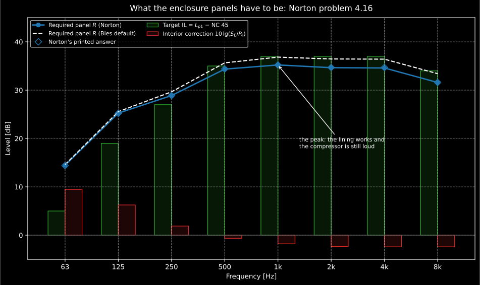
Octave-band chart from 63 Hz to 8 kHz of Norton problem 4.16. Green bars give the target insertion loss, rising from 5 dB at 63 Hz to 37 dB from 1 kHz to 4 kHz; red bars give the interior correction, falling from plus 9.5 dB at 63 Hz through zero near 400 Hz to about minus 2.4 dB above 2 kHz; and the required panel transmission loss runs as a curve peaking at 35.2 dB at 1 kHz and falling to 14.5 dB at 63 Hz and 31.6 dB at 8 kHz, with Norton's printed answers marked as open diamonds on it and the library's default Bies model drawn dashed a decibel or two above from 500 Hz upwards

The requirement is the sum of the two bar families, and they peak in different places: the target insertion loss keeps climbing to 1 kHz while the interior correction falls from +9.5 dB at 63 Hz, where a 50 mm blanket is acoustically thin, to −2.4 dB above 2 kHz, where the lining has taken the interior room constant past the radiating area. The dashed Bies default carries the 0.3 floor discussed below and sits up to 1.8 dB above Norton’s model once the lining dominates.

Show the code for this figure

import matplotlib.pyplot as plt

# `required` is the EnclosureResult built above.

# One line: the target IL, the interior correction and the required panel R.
required.plot()
plt.show()

# By hand, from the per-band fields the result carries:
fig, ax = plt.subplots()
ax.semilogx(required.frequencies, required.insertion_loss, "s--",
            label="Target IL")
ax.semilogx(required.frequencies, required.correction, "^:",
            label="Interior correction")
ax.semilogx(required.frequencies, required.panel_transmission_loss, "o-",
            label="Required panel R")
ax.set_xlabel("Frequency [Hz]"); ax.set_ylabel("Level [dB]")
ax.legend()
plt.show()

Two footnotes on that snippet, both about being faithful to the source. model="norton" matters: the library’s default enclosure model is Bies, Hansen & Howard’s Equation (7.111), which carries a $0.3$ inside the logarithm and so floors the insertion loss of a fully lined enclosure at $TL + 5.2 dB$ . Norton’s Equation (4.115) has no such floor. The two agree within a few tenths while the interior is hard and diverge once the lining takes over, and reproducing a published answer means using the model its author used. ENCLOSURE_MODELS lists both.

And the NC-45 column is Norton’s own, taken from his problem statement. It reads 41 dB in the 8 kHz band where ANSI/ASA S12.2-2019 Table 1 (which nc_curve implements) reads 42 dB; they agree in every other band. Using the printed column keeps the oracle the published one.

One caveat carries over from section 6 and bites harder here. The required panel transmission loss is an upper bound in exactly the way the partition’s is, and for sharper reasons: an enclosure is small, so the ratio of its unavoidable openings — access door, cable and pipe entries, cooling apertures, conveyor slots — to its total area is far higher than a wall’s, and an open fraction of one per cent caps the achieved insertion loss near 20 dB whatever the 35 dB panel this calculation asks for. The machine must also not touch the enclosure or share its base: a bolted contact radiates the machine’s vibration from the outer skin and bypasses the panels entirely. Put the openings into the calculation rather than hoping — the composite route and the drawn construction are in Industrial noise control §2.1 — and use the same flanking_penalty below as the honest place to record whatever is left unmodelled.

6. What the prediction does not know

Norton’s answer to problem 4.21 ends with the caveat that matters more than any of the arithmetic above: the measured noise reduction runs below the prediction because of flanking transmission through mechanical connections and air leaks. A ceiling void carried over the partition, a service penetration, a door undercut, or the wall simply not reaching the structural slab, and the equation’s answer becomes an upper bound.

The clip below draws what the equation leaves out. The chain of section 3 prices the direct path only, the Dd route through the partition; the other three pulses leave the source room over the flanking walls, floor or ceiling — Ff flank to flank, Fd flank to partition, Df partition to flank — and re-radiate on the far side without ever passing through the transmission loss the calculation used. Each path shrinks at every element and junction it crosses, which is why no single one has to be large for the sum of the three to dominate a good partition.

Download the animation (WebM)

DesignCriterion.flanking_penalty is the explicit debit for that, in decibels off the predicted noise reduction. It is not a model, it is a place to record the allowance and have it show up in .table() and in the required transmission loss rather than get lost:

# The chain of section 3 again, with 3 dB allowed for flanking and leaks.
honest = room_to_room_transmission(
    bands, [39.0, 42.0, 50.0, 58.0, 63.0, 67.0], 15.0,
    equivalent_absorption_area(operator),
    source=SourceRoom(level=chain.source_level),
    criterion=DesignCriterion(target=45.0, flanking_penalty=3.0),
)
print(np.round(honest.received_level, 1))
# [75.4 63.4 44.4 44.  36.9 33.7]      every band 3 dB worse

Where the flanking paths are modelled rather than allowed for, the prediction models of EN 12354 are the right tool, and those live in Building sound insulation prediction and Flanking transmission.

The other assumption is diffusivity, and it fails in two directions. In frequency: Equation (4.101) is a diffuse-field balance in both rooms, so it has nothing to say below each room’s Schroeder frequency (schroeder_frequency), where discrete modes rule. The 5 m × 5 m × 3 m operator room above, 75 m³, has a Schroeder frequency of 163 Hz for a half-second reverberation time, which is exactly why the 125 Hz band of problem 4.18 — the band that governs the whole answer — should be read as an estimate and not as a number. The call is schroeder_frequency(0.5, 75.0), reverberation time first and volume second, and it returns 163.3 Hz for that room.

In space: both levels are reverberant-field spatial averages. $L_{p 2}$ is what a roving microphone would report over the receiving room, not the level at the desk pushed against the party wall, where the direct field of the radiating surface adds a few decibels within roughly a wavelength of it. The same holds in reverse on the source side — $L_{p 1}$ is the reverberant level that drives the whole partition, and a person standing beside the machine is in its direct field and hears more, so a measured source-room level has to be taken away from both the machine and the wall to be the right input. It is the reason the field standards keep their microphone positions half a wavelength from every surface, and the reason this calculation cannot answer where in the receiving room to put the workstation; when that is the question, the image-source and ray methods of Room image sources and steady field are the tool.

What this guide covers

Covered
The Norton & Karczub §4.9 power balance (Eq. 4.101) as room_to_room_transmission, with SourceRoom, equivalent_absorption_area, mean_absorption and room_constant; the source-room level from a sound power level through the §4.6 Table 4.5 source models (constant power, constant volume, constant pressure) and the directivity of the machine’s position; DesignCriterion with its target, its flanking allowance and its ANSI/ASA S12.2-2019 rating, in the NC family by default and in the RC Mark II family with DesignCriterion(family="RC"); .required_transmission_loss, .exceedance, .meets_target and .table(); and the §4.10 enclosure equation (Eq. 4.115) through enclosure_required_transmission_loss, in both the Norton and the Bies interior models listed by ENCLOSURE_MODELS.
Not covered
The transmission loss of the partition itself, which is measured or predicted elsewhere; flanking as a modelled path rather than a flat allowance; the leaks and openings of an enclosure, which need the composite of the industrial noise-control guide; and anything below each room’s Schroeder frequency, or closer to a surface than about half a wavelength.

References

American National Standards Institute. (2019). Criteria for evaluating room noise (ANSI/ASA S12.2-2019). The NC curves of Table 1 and the RC Mark II family of Annex D that the chain is rated against.
Bies, D. A., Hansen, C. H., & Howard, C. Q. (2017). Engineering noise control (5th ed.). CRC Press. https://doi.org/10.1201/9781351228152The steady-state room relations (section 6.4, Eqs. 6.43-6.44) behind steady_state_spl and room_constant, and the enclosure insertion loss of section 7.4.2 (Eqs. 7.103, 7.111) that is the library default enclosure model.
Kuttruff, H. (2016). Room acoustics (6th ed.). CRC Press. The Schroeder frequency (Eq. 3.44) that bounds the diffuse-field assumption from below.
Norton, M. P., & Karczub, D. G. (2003). Fundamentals of noise and vibration analysis for engineers (2nd ed.). Cambridge University Press. https://doi.org/10.1017/CBO9781139163927The sound power models of section 4.6 (Table 4.5, Eqs. 4.53-4.56), the room-to-room power balance of section 4.9 (Eqs. 4.92-4.101), the enclosure design equation of section 4.10 (Eqs. 4.102-4.115) and the worked problems 4.16, 4.18 and 4.21 with their printed octave-band answers, which this guide is built around.

Created and maintained by José Manuel Requena Plens ORCID All projects

Room to Room: Partition, Receiving Room, Criterion

1. What the balance says

What a measurement of the same pair reports

2. Three partitions, one receiving room

3. The chain, end to end

4. The verdict, and the number to specify

5. An enclosure against a criterion

6. What the prediction does not know

What this guide covers

See also

References