Microphone Characterisation (IEC 60268-4)

Every acoustic measurement in this documentation starts at a microphone, and IEC 60268-4 is the standard that fixes how the device itself is described: what its sensitivity refers to, how its directional pattern is stated, and how its self-noise and overload point bound the levels it can read. This guide covers the conventions where datasheet comparisons go wrong (the sensitivity references and the noise weightings), the directional patterns with their directivity index, and the rated-characteristics report that renders the standard’s data sheet from a measured free-field response, with every panel drawn to the IEC 60263 scale conventions. The distortion and frequency-response measurements themselves live in Electroacoustics; the loudspeaker counterpart has its own guide.

1. Sensitivity and its references (IEC 60268-4 clause 11)

The sensitivity $M$ is the output voltage per unit sound pressure, quoted in mV/Pa; the sensitivity level is $L_M=20{\log }_{10}(M/1\text{V/Pa})$ dB, which is negative for every real microphone (a 50 mV/Pa studio condenser sits at −26 dB re 1 V/Pa). The classic pitfall is the reference: −26 dB re 1 V/Pa and +34 dB re 1 mV/Pa are the same microphone, 60 dB apart on paper, so a sensitivity level without its reference is meaningless. The standard also distinguishes free-field, diffuse-field and pressure sensitivity; for the same capsule they diverge at high frequency, so the stated type matters as much as the number.

Behind the number sits the transducer. A condenser capsule (externally polarised or electret) reads the sound pressure as a capacitance change and needs powering, but converts with high sensitivity, typically some tens of mV/Pa for a studio diaphragm and a few mV/Pa for a small measurement capsule; virtually every measurement microphone is a condenser because the stretched-membrane capsule is stable enough to calibrate. A dynamic (moving-coil) microphone generates its voltage by induction, needs no power and survives abuse, but converts far less efficiently, around 1-3 mV/Pa, which is why a dynamic on a quiet source runs out of preamplifier gain before a condenser does. The rated sensitivity of the standard is quoted at the 1 kHz reference frequency (clause 11.3), into the rated load, and the stated type (free-field, diffuse-field or pressure) is part of the rating, not a detail.

1.1 The three sensitivity types, and how to choose one

The three types differ only in the field the capsule is calibrated in, and they exist because a microphone is not a point. At frequencies where the capsule is no longer small against the wavelength it perturbs the field it is measuring, and the pressure on the diaphragm rises above the undisturbed pressure for sound arriving on the reference axis — by several decibels for a half-inch capsule above about 5 kHz, and higher still for a quarter-inch one. The three definitions are three ways of dealing with that:

• Pressure sensitivity (11.2.4) is the ratio of output voltage to the sound pressure actually present at the acoustic entry. It is what a coupler, a pistonphone or an electrostatic actuator realises, and what a capsule flush in a boundary reads.
• Free-field sensitivity (11.2.1) is referred to the undisturbed pressure of a plane progressive wave arriving on the reference axis, so the capsule’s own pressure build-up is corrected out.
• Diffuse-field sensitivity (11.2.2) is referred to sound arriving from all directions with random phase; the standard defines it as the r.m.s. of the free-field sensitivities over all directions, so $L_{M,\text{diff}}=L_{M,\text{ff}}-D$ with $D$ the directivity index of section 2.

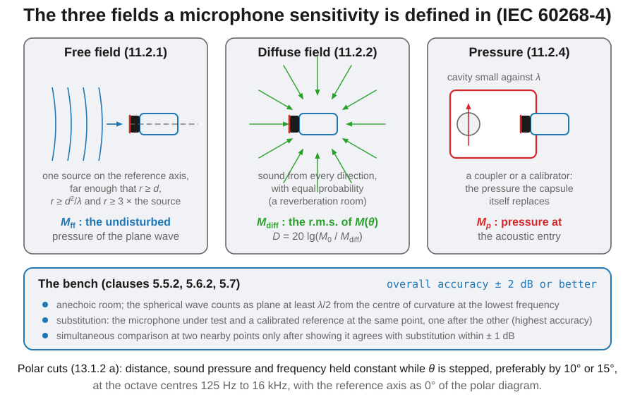
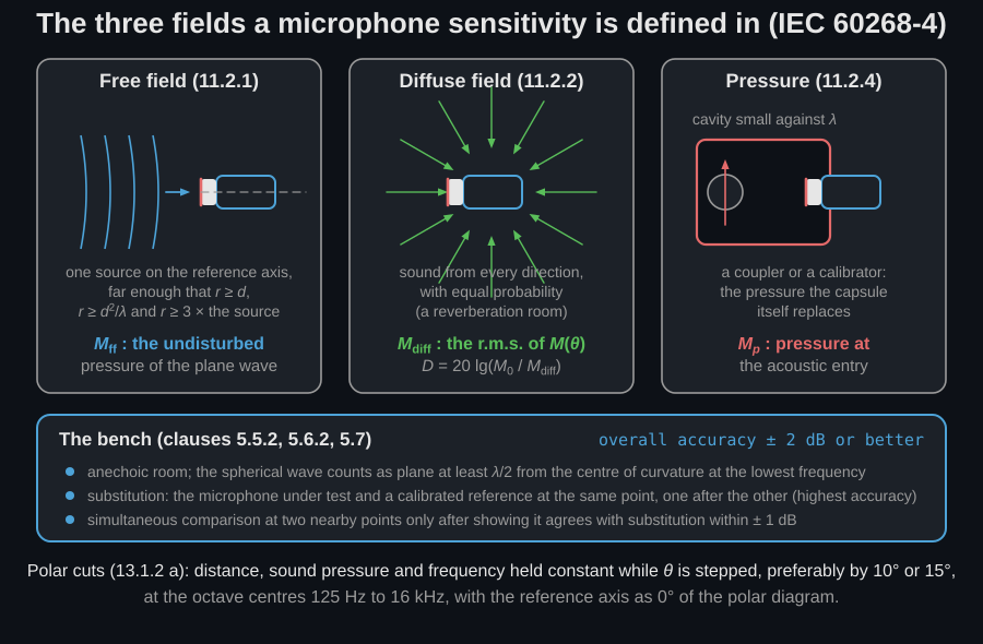
The selection rule. A free-field capsule pointed at a known source in a free or near-free field; a random-incidence capsule in a reverberant room, and for an IEC 61672 class 1 sound level meter used indoors; a pressure capsule in a coupler or flush in a boundary. Using a free-field capsule at grazing incidence, or a pressure capsule on axis, costs several decibels in the top two octaves and nothing at all below 1 kHz — which is why the error survives an A-weighted level check and appears only in a spectrum. The size trade-off runs the other way: a smaller capsule keeps its field type honest to a higher frequency and pays for it in sensitivity and self-noise.

The bench behind the number. IEC 60268-4 clause 4.2.2 defines rated conditions for a microphone: the specified resistive load, the rated power supply, a free field (5.5.2) at zero degrees to the reference direction, and an undisturbed sound pressure of 1 Pa (94 dB) at the reference point, at the 1 kHz measurement frequency. Clause 5.5.2 fixes the geometry: free-field conditions realised in the open air, in an anechoic room or in a duct, with the spherical-wave referral valid only where $r\ge d$ and $r\ge d^2/\lambda$ for an effective source diameter $d$ — preferably beyond three times the largest dimension of the radiating surface — and a spherical wave counted as plane only at least half a wavelength from its centre of curvature at the lowest measured frequency. Clause 5.6.2 fixes the calibration: the substitution method, in which the microphone under test and a calibrated reference occupy the same point one after the other, gives the highest accuracy; the simultaneous comparison at two nearby points may be used only after showing it agrees with substitution within ±1 dB. Clause 5.7 caps the whole thing: an overall accuracy of ±2 dB or better shall be obtained. Every number in the fiche of section 4 inherits that bound. Turning a rated sensitivity into calibrated levels on a working chain is Calibration and dBFS.

2. Directional pattern and the directivity index (clause 13)

The directional response is stated as the pattern of sensitivity against the angle of incidence, normalized to the reference axis. The classic first-order family mixes an omnidirectional (pressure) term and a cosine (pressure-gradient) term, $M(\theta )\propto (1-b)+b\cos \theta$: $b=0$ is the omnidirectional capsule, $b=1/2$ the cardioid with its null at 180°, and $b=1$ the figure-of-eight with nulls at ±90°. One number condenses the pattern: the directivity index $D=20{\log }_{10}(M_0/M_{\mathrm{diff}})$ compares the reference-axis sensitivity with the diffuse-field sensitivity obtained from the clause 11.2.2 a) integral over a rotationally symmetric pattern (clause 13.2.2; the index is anchored on two clauses because the $M_{\mathrm{diff}}$ it divides by is the one clause 11.2.2 a) defines, as the r.m.s. of the pattern over a rotationally symmetric solid angle). An omni scores 0 dB, the ideal cardioid and figure-of-eight both $10{\log }_{10}3=4.8$ dB: in a diffuse room field, a cardioid picks up three times less reverberant power than an omni of equal axial sensitivity, which is exactly the ratio a talker-to-microphone distance calculation wants. Real patterns hold their textbook shape only over the middle of the band; at high frequency the capsule’s own size makes any microphone directive, which is also why the free-field and diffuse-field sensitivities of one capsule diverge there.

The whole family is six values of one coefficient. The directivity indices below are what microphone_characteristics returns for each pattern through the clause 11.2.2 a) integral (the section-4 snippet prints three of them), and the random-energy efficiency is the fraction of a diffuse field the capsule still picks up:

Pattern	$b$	$M(180°)$	Null	Directivity index	Random-energy efficiency	Distance factor
Omnidirectional	0	+1.00	—	0.0 dB	1.000	1.00
Subcardioid	1/3	+0.33	—	3.2 dB	0.481	1.44
Cardioid	1/2	0.00	180°	4.8 dB	0.333	1.73
Supercardioid	0.63	−0.26	126°	5.7 dB	0.269	1.93
Hypercardioid	3/4	−0.50	110°	6.0 dB	0.250	2.00
Figure-of-eight	1	−1.00	±90°	4.8 dB	0.333	1.73

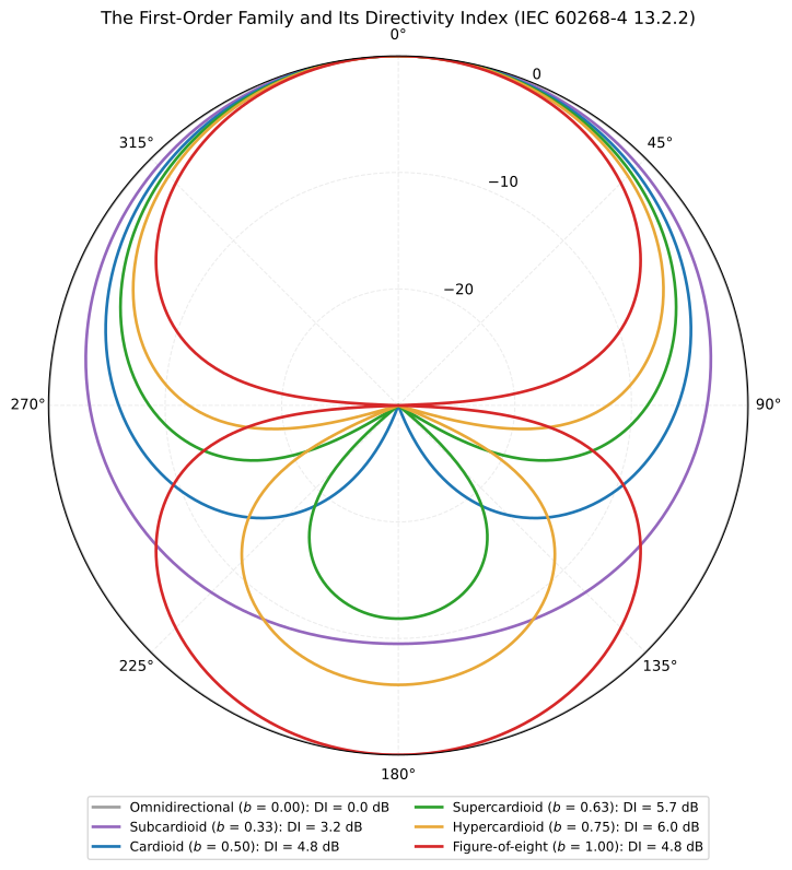
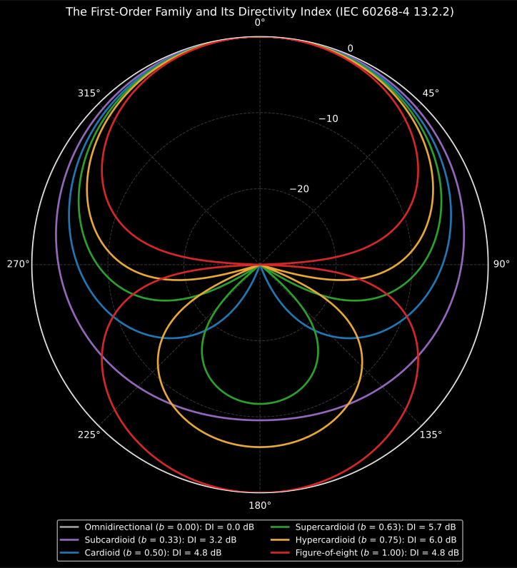
The cardioid and the figure-of-eight return the same 4.8 dB from opposite geometries: the index says how much reverberant power a capsule rejects, not from where. That is why a pattern and an index are always quoted together, and why the supercardioid and hypercardioid — which trade a rear lobe for a deeper null off-axis — beat both on the number while sounding quite different behind. The distance factor is the practical consequence: a cardioid may sit 1.73 times further from a talker than an omnidirectional capsule for the same direct-to-reverberant ratio.

Show the code for this figure

import matplotlib.pyplot as plt
import numpy as np

# The pattern shapes. The directivity index annotated on each curve is the
# one `microphone_characteristics(...).directivity_index_db` returns for the
# same polar data, as in the snippet of section 4.
theta = np.radians(np.linspace(0.0, 360.0, 721))
ax = plt.subplot(projection="polar")
for b in (0.0, 1 / 3, 0.5, 0.63, 0.75, 1.0):
    mag = np.maximum(np.abs((1.0 - b) + b * np.cos(theta)), 10 ** (-1.5))
    ax.plot(theta, np.maximum(20 * np.log10(mag), -30.0))
ax.set_ylim(-30.0, 0.0)
plt.show()

The cosine term is a pressure-gradient term, and that has a consequence the formula hides: close to a source the gradient carries a component that grows as $1/r^2$ while the pressure term falls as $1/r$, so any capsule with $b>0$ boosts low frequencies as it approaches the source. The proximity effect is typically 6 to 10 dB at 100 Hz at 5 cm for a cardioid and larger for a figure-of-eight. It is exploited deliberately in speech work, and it is the reason a directional microphone cannot be used as a measurement device near a source: the response depends on where it is held. Together with the frequency dependence of a real pattern, that is why every measurement microphone in this documentation is an omnidirectional pressure capsule.

3. Inherent noise: dB(A) and dB(468) (clause 17)

A microphone’s electronics and the air load on its diaphragm set a noise floor, expressed as the equivalent noise level: the sound pressure level whose output would equal the weighted inherent-noise voltage, $L_N=20{\log }_{10}((U_N/M)/20\mu \text{Pa})$. The standard states it with two weightings, and the numbers are far apart on paper. The A-weighted figure (RMS detector) is the one most datasheets quote, e.g. 14 dB(A) for a good studio condenser. The ITU-R BS.468-4 figure weights the same noise with the curve that peaks +12.2 dB near 6.3 kHz and reads it with a quasi-peak detector, so it penalises the hiss and crackle the ear actually notices; for typical microphone noise it comes out roughly 10 dB above the A-weighted number for the same capsule. Neither is wrong: they are different weightings of the same voltage, and comparing a dB(A) figure from one datasheet with a dB(468) figure from another silently flatters the first by that margin. The signal-to-noise ratio re 1 Pa (94 dB SPL) is derived from the same equivalent noise level, and the overload sound pressure level (clause 15.2) bounds the usable range from above. The BS.468 weighting curve itself is exposed as itu_r_468_weighting in the electroacoustics distortion set, where it also weights THD.

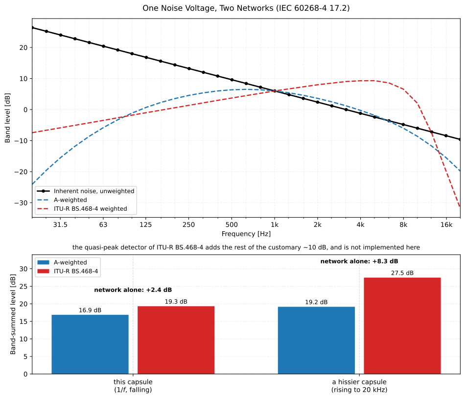
How much of the gap the network alone accounts for depends on the shape of that capsule’s noise: 2.4 dB for the falling 1/f spectrum of the example, 8.3 dB for a hissier capsule. The rest of the customary 10 dB comes from the ITU-R 468 quasi-peak detector, which reads a noise higher than an r.m.s. detector does; itu_r_468_weighting is the network only, so a level computed with it and an r.m.s. sum is not a dBqps figure and must not be compared with one from a datasheet.

The band spectrum drawn there is the one the section-4 snippet passes as MicrophoneNoise(spectrum=...), weighted with itu_r_468_weighting from the electroacoustics module and with A-weighting, then summed band by band.

How $U_N$ is obtained (clause 17.2). The microphone is isolated from sound, wind, shock, vibration and electric or magnetic fields, but it must stay in acoustical operating mode: the standard warns explicitly that replacing the transducer element with an equivalent circuit does not measure the microphone, because the element contributes noise of its own. A 40 to 60 dB preamplifier keeps the microphone’s own noise dominant, so no correction for the instrumentation is needed. Then comes the check that decides whether the number is usable: replace the microphone with a resistor at room temperature equal to its rated impedance and require the measured output to be less than one third of the value measured with the microphone, so that the instrumentation and any residual external sound inflate the result by less than 10 %. Report which weighting and detector produced the figure — A-weighted r.m.s. (IEC 60268-1 6.2.1), ITU-R 468 quasi-peak (6.2.2), or unweighted third octaves (6.2.3) — because the three differ by about 10 dB on the same capsule and the clause asks for the quasi-peak measurement to be among them.

3.1 What else bounds the usable range

The overload sound pressure level (15.2) is the pressure of a plane wave at which the microphone’s amplitude non-linearity reaches a declared limit, for any frequency in the effective range and any direction of incidence; the standard notes that no common limit exists and that data sheets typically declare 0.5 % or 1 %. Producing the field is the hard part of the measurement: a 140 dB level has to come from something whose own distortion is well below the capsule’s — in practice a small pressure chamber or a compression driver on a coupler, with the source’s own distortion characterised first against a reference microphone. Sweep the level with an ordinary loudspeaker and the curve plotted is the loudspeaker’s. The clause’s own way round the problem is to use the difference-frequency measurement of 14.4.2 instead, which at least minimises the influence of the source’s non-linearity.

Three further limits are rated characteristics in their own right, and all three are quoted as equivalent sound pressure levels, so they can be compared band for band with the inherent noise above:

• Mechanical vibration (19.2): the equivalent sound pressure produced by a stated r.m.s. acceleration in the direction of maximum influence, with the direction of minimum influence also stated, measured with a gliding frequency up to 250 Hz. This is stand and handling noise, and it is why a shock mount is specified rather than assumed.
• Wind (19.3): the equivalent sound pressure for a stated wind velocity and direction, the reference value being 10 m/s. It is the quantity a windscreen’s effectiveness is stated against.
• Transient “pop” effect (19.4): the plosive burst of a close talker, which a pop filter or a change of working distance addresses.

4. Microphone characteristics report (IEC 60268-4)

The microphone companion of the loudspeaker report: the rated characteristics IEC 60268-4 defines around a measured free-field frequency response are gathered into a single microphone characteristics result that renders the standard’s rated-characteristics data sheet. Four of the numbers are computed from the standard’s own definitions rather than merely repeated:

• Sensitivity level (11.1). The rated free-field sensitivity $M$ (mV/Pa, at the 1 kHz reference frequency of 11.3) as a level, $L_M=20{\log }_{10}(M/1\text{V/Pa})$: 12.5 mV/Pa is $-38.1$ dB re 1 V/Pa.
• Effective frequency range (12.2). The band over which the response, normalized to 0 dB at the reference frequency, stays within the stated $\pm$ tolerance; the edges are the interpolated tolerance crossings.
• Directivity index (13.2.2). $D=20{\log }_{10}(M_0/M_{\mathrm{diff}})$ with the diffuse-field sensitivity from the 11.2.2 a) integral over a rotationally symmetric pattern; the ideal cardioid returns $10{\log }_{10}3=4.8$ dB.
• Equivalent noise level (17.2). The weighted inherent-noise voltage over the rated sensitivity as a sound pressure level, $L_N=20{\log }_{10}((U_N/M)/20\mu \text{Pa})$, with the signal-to-noise ratio re 1 Pa (94 dB SPL) derived from it. The overload sound pressure level (15.2) is read from a distortion-against-level curve at the stated THD limit.

The four input curves in the snippet below are synthetic, but each stands for a named measurement and it is worth knowing which before collecting data. The free-field response comes from a substitution calibration against a reference microphone in an anechoic room (5.6.2 a), or is synthesised from an electrostatic-actuator pressure response plus the manufacturer’s free-field correction, and is normalised to 0 dB at the 1 kHz reference frequency the report marks. The polar cuts come from rotating the microphone on a turntable in the same room, one cut per stated frequency, in a plane containing the reference axis, with the distance, the sound pressure and the frequency held constant while $\theta$ is stepped (13.1.2 a). The inherent-noise spectrum is the third-octave breakdown of the clause 17.2 measurement, with the analyser bandwidth stated, and the single voltage is the weighted r.m.s. of the same measurement. The distortion-against-level curve comes from stepping the sound pressure of a high-level source while the distortion at the output is measured (15.2.2), and the overload level is read off it where the curve crosses the declared limit.

import numpy as np
from phonometry import (
    MicrophoneDirectivity, MicrophoneElectrical, MicrophoneNoise,
    MicrophoneOverload, ReportMetadata, microphone_characteristics,
)

freqs = np.geomspace(20, 20000, 400)
response = -10 * np.log10(1 + (30.0 / freqs) ** 4)      # low-frequency roll-off
response -= 10 * np.log10(1 + (freqs / 19000.0) ** 8)   # high-frequency roll-off
response += 2.0 * np.exp(-(np.log2(freqs / 9000.0) ** 2) / 0.3)  # presence region

angles = np.linspace(0, 179, 359)
cardioid = 20 * np.log10((1 + np.cos(np.radians(angles))) / 2)
noise_f = np.geomspace(20, 20000, 31)

result = microphone_characteristics(
    freqs, response, 12.5, tolerance_db=3.0,          # 12.5 mV/Pa at 1 kHz
    directivity=MicrophoneDirectivity(polar=(angles, cardioid), frequency=1000.0),
    noise=MicrophoneNoise(                             # A-weighted, V
        voltage=1.25e-6,
        spectrum=(noise_f, 6.0 + 12.0 * np.log10(1000.0 / noise_f)),
    ),
    overload=MicrophoneOverload(
        distortion=(np.linspace(100, 140, 81),
                    0.5 * 10 ** ((np.linspace(100, 140, 81) - 130.0) * 0.08)),
        thd_percent=0.5,
    ),
    electrical=MicrophoneElectrical(
        rated_impedance=150.0, minimum_load_impedance=1000.0,
        powering="Phantom P48 (IEC 61938)", supply_current_ma=3.1,
    ),
)
print(round(result.sensitivity_level_db, 1))            # -38.1 dB re 1 V/Pa
print(tuple(round(x) for x in result.effective_range))  # Hz
print(round(result.directivity_index_db, 1))            # 4.8 dB (cardioid)
print(round(result.equivalent_noise_level_db, 1))       # 14.0 dB(A)
print(round(result.signal_to_noise_ratio_db, 1))        # 80.0 dB re 1 Pa

# The three canonical patterns of section 2, through the same 11.2.2 a)
# integral: b = 1/2 and b = 1 return the same index from opposite shapes.
for b in (0.0, 0.5, 1.0):
    polar = 20 * np.log10(
        np.maximum(np.abs((1 - b) + b * np.cos(np.radians(angles))), 1e-3))
    family = microphone_characteristics(
        freqs, response, 12.5, tolerance_db=3.0,
        directivity=MicrophoneDirectivity(polar=(angles, polar),
                                          frequency=1000.0))
    print(b, round(family.directivity_index_db, 1))     # 0.0 / 4.8 / 4.8 dB

result.report("microphone.pdf", metadata=ReportMetadata(measurement_standard="IEC 60268-4"))

The fourth print closes a chain the page has left open twice. An inherent-noise voltage of 1.25 µV at the output of a 12.5 mV/Pa capsule is an acoustic pressure of 100 µPa at its diaphragm, which is $20{\log }_{10}(100/20)=14.0$ dB above the 20 µPa reference: this microphone would read 14 dB(A) in a perfectly silent room, and cannot measure anything quieter than about 24 dB(A) without contributing to the answer. The signal-to-noise ratio the result also carries is simply 94 dB minus that figure — 80.0 dB — because the standard’s reference is 1 Pa. The same voltage read through ITU-R BS.468-4 with a quasi-peak detector would be reported about 10 dB higher for the same capsule, so this number is 14 dB(A) and must never be set beside a dB(468) figure from another sheet.

One trap the API reproduces and the page has to close: MicrophoneNoise.voltage is the inherent-noise voltage as measured through the weighting network, not a raw wideband r.m.s., and weighting= records which network that was. It defaults silently to 'A' (IEC 60268-1 6.2.1). The field is a label, not a filter: the function re-weights nothing, so declaring weighting="CCIR" while passing an A-weighted voltage produces a correctly computed level with the wrong name on it — exactly the error section 3 warns about, now printed on a report. Quoting both figures for the same capsule is the honest form, since they are different questions and both are legitimate.

microphone_characteristics returns a MicrophoneCharacteristics with the computed sensitivity_level_db, effective_range, directivity_index_db, equivalent_noise_level_db, max_spl_db, signal_to_noise_ratio_db and diffuse_field_sensitivity_level_db, and a .report() that writes the fiche. The free-field response is drawn with its tolerance band, the reference-frequency marker and the effective-range markers to the IEC 60263 proportion (one frequency decade equal to 25 dB), and the directional pattern on the IEC 60263 25 dB reference circle; the inherent-noise spectrum and the distortion-against-level curve (with the THD limit and the overload level marked) feed the secondary panels. A requirement in the metadata is checked as a maximum permitted equivalent noise level.

The rated characteristics are also available interactively through .plot(), which draws one concept per figure with the same panel code the report composes, selected by quantity. Passing an axes draws on it:

result.plot()                        # free-field response (default)
result.plot(quantity="directivity")  # polar pattern on the 25 dB circle
result.plot(quantity="noise")        # inherent-noise band spectrum
result.plot(quantity="distortion")   # THD vs sound pressure level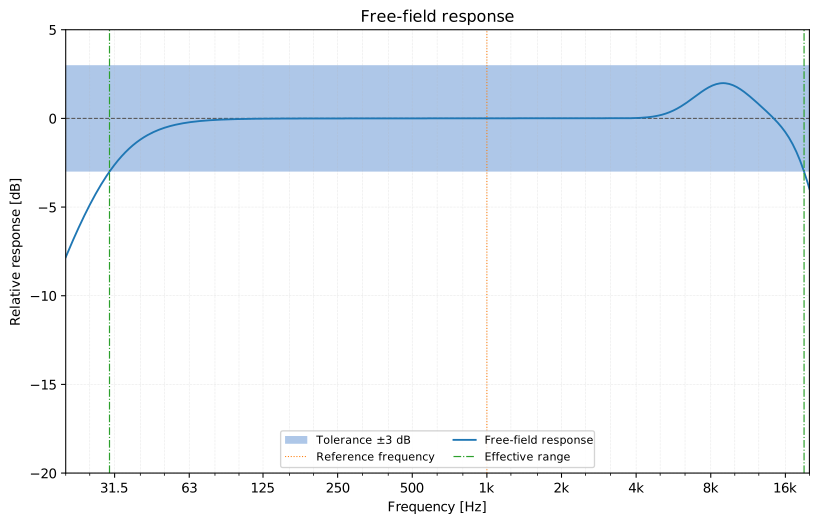

The shaded band is the tolerance the reader declares (tolerance_db, 3 dB here) and the effective-range edges of clause 12.2 are its interpolated crossings, so a tighter tolerance shortens the quoted range: two microphones cannot be compared on range alone without it. The curve is normalised to 0 dB at the 1 kHz reference frequency of clause 11.3, which is where the rated sensitivity is quoted, and the lift near 9 kHz here is a deliberate presence peak rather than a defect.

Show the code for this figure

import matplotlib.pyplot as plt
import numpy as np
from phonometry import microphone_characteristics

freqs = np.geomspace(20, 20000, 400)
response = -10 * np.log10(1 + (30.0 / freqs) ** 4)      # low-frequency roll-off
response -= 10 * np.log10(1 + (freqs / 19000.0) ** 8)   # high-frequency roll-off
response += 2.0 * np.exp(-(np.log2(freqs / 9000.0) ** 2) / 0.3)  # presence region

result = microphone_characteristics(freqs, response, 12.5, tolerance_db=3.0)
result.plot()   # quantity="response" (the default)
plt.show()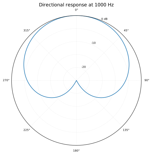

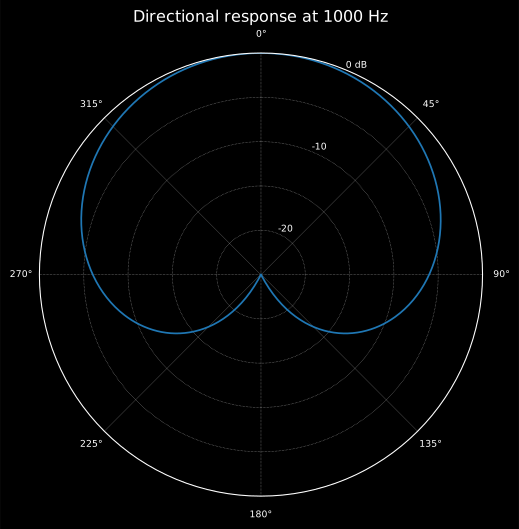
Drawn on the IEC 60263 25 dB reference circle of clause 3, so the full radius is 25 dB and each ring is 5 dB; the cardioid’s rear rejection is the depth of its 180° null. This is one cut at one frequency — a real capsule holds the textbook shape only through the middle of its band, which is why clause 13.1.2 a) asks for the octave centres from 125 Hz to 16 kHz. It is the panel the 4.8 dB directivity index of the fiche is computed from.

Show the code for this figure

import matplotlib.pyplot as plt
import numpy as np
from phonometry import MicrophoneDirectivity, microphone_characteristics

freqs = np.geomspace(20, 20000, 400)
response = -10 * np.log10(1 + (30.0 / freqs) ** 4)
angles = np.linspace(0, 179, 359)
cardioid = 20 * np.log10((1 + np.cos(np.radians(angles))) / 2)

result = microphone_characteristics(
    freqs, response, 12.5, tolerance_db=3.0,
    directivity=MicrophoneDirectivity(polar=(angles, cardioid), frequency=1000.0),
)
result.plot(quantity="directivity")
plt.show()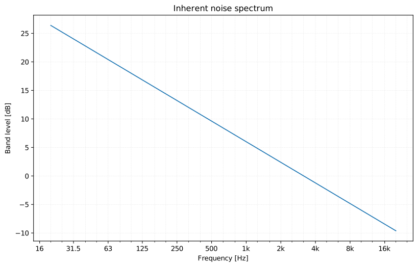

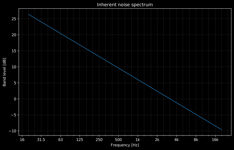
The band breakdown behind the single equivalent-noise figure, and note the ordinate: these are equivalent sound pressure band levels, not voltages. The rising low-frequency end is the amplifier’s 1/f noise, which A-weighting discounts heavily, which is why the A-weighted total is dominated by the mid bands and why the same capsule reads so differently through the 468 network.

Show the code for this figure

import matplotlib.pyplot as plt
import numpy as np
from phonometry import MicrophoneNoise, microphone_characteristics

freqs = np.geomspace(20, 20000, 400)
response = -10 * np.log10(1 + (30.0 / freqs) ** 4)
noise_f = np.geomspace(20, 20000, 31)

result = microphone_characteristics(
    freqs, response, 12.5, tolerance_db=3.0,
    noise=MicrophoneNoise(
        voltage=1.25e-6,
        spectrum=(noise_f, 6.0 + 12.0 * np.log10(1000.0 / noise_f)),
    ),
)
result.plot(quantity="noise")
plt.show()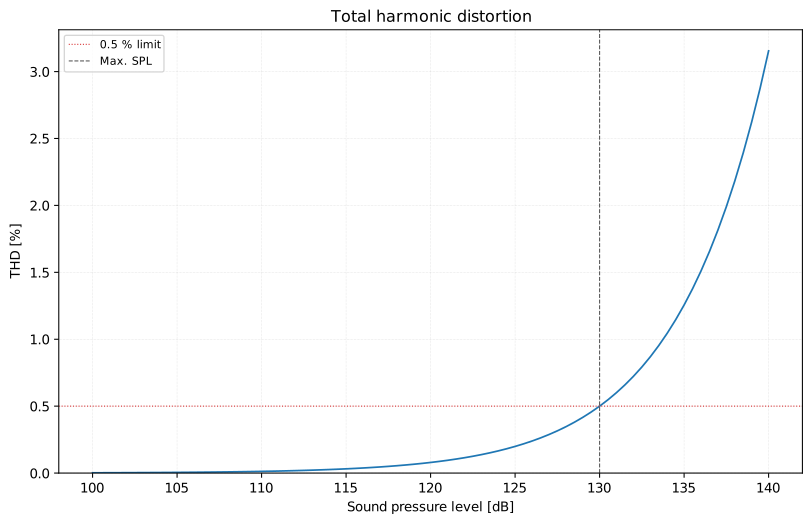

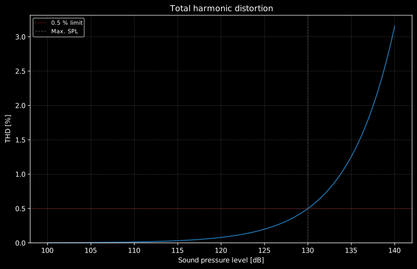
The knee is where the capsule’s motion stops being linear, and the overload sound pressure level of clause 15.2 is simply the reading of this curve at the declared limit — so a “max SPL” quoted at 0.5 % and one quoted at 3 % differ by several decibels for the same microphone, and neither means anything without its percentage.

Show the code for this figure

import matplotlib.pyplot as plt
import numpy as np
from phonometry import MicrophoneOverload, microphone_characteristics

freqs = np.geomspace(20, 20000, 400)
response = -10 * np.log10(1 + (30.0 / freqs) ** 4)
spl_axis = np.linspace(100, 140, 81)

result = microphone_characteristics(
    freqs, response, 12.5, tolerance_db=3.0,
    overload=MicrophoneOverload(
        distortion=(spl_axis, 0.5 * 10 ** ((spl_axis - 130.0) * 0.08)),
        thd_percent=0.5,
    ),
)
result.plot(quantity="distortion")
plt.show()

The example fiche is regenerated with make reports and kept rendered in the repository; click the preview to open the PDF.

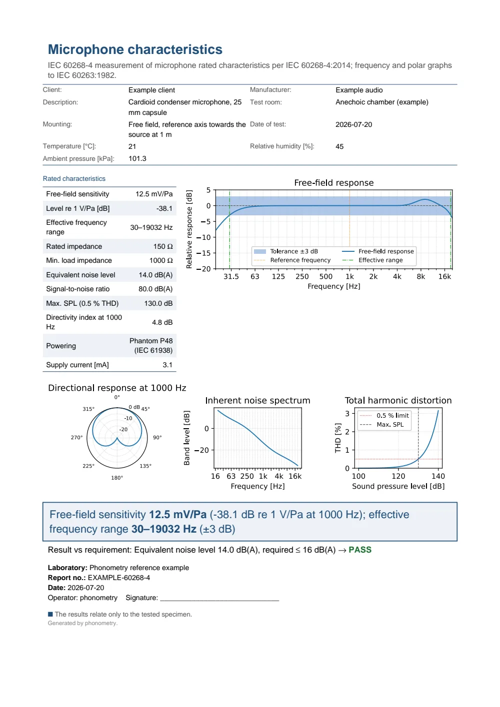
One-page IEC 60268-4 microphone rated-characteristics fiche: a header with the manufacturer and model, the rated-characteristics table (free-field sensitivity in mV/Pa and its level re 1 V/Pa, effective frequency range, rated and minimum load impedances, equivalent noise level, signal-to-noise ratio, maximum SPL at the stated THD limit, directivity index and phantom powering) beside the free-field frequency response with its tolerance band and effective-range markers, and the directional-pattern, inherent-noise-spectrum and distortion panels, all drawn to the IEC 60263 scale conventions.

Download the report (PDF)

Microphone characteristics fiche (MicrophoneCharacteristics.report), the IEC 60268-4 rated-characteristics table beside the free-field response, with the cardioid directional pattern, inherent-noise and THD-against-level panels drawn to the IEC 60263 25 dB-per-decade and 25 dB reference-circle conventions.

What this guide covers

• Covered

  The three sensitivity types and the rated conditions, geometry, substitution calibration and ±2 dB accuracy bound behind them (clauses 4.2.2, 5.5.2, 5.6.2, 5.7, 11.2), the clause 17.2 inherent-noise procedure with its one-third residual check, and the clause 15.2/19.2-19.4 limits. The IEC 60268-4:2014 rated microphone characteristics via microphone_characteristics and its .report(): the sensitivity level re 1 V/Pa (11.1/11.3), the effective frequency range against a stated tolerance (12.2), the directivity index through the 11.2.2 a) diffuse-field integral (13.2.2), the equivalent noise level and signal-to-noise ratio (17.2), the overload sound pressure level read off a distortion curve (15.2) and the rated impedances and powering (9/10), with the response, polar, noise and distortion panels drawn to the IEC 60263 scale conventions.

• Not covered

  The laboratory’s own instrumentation: the anechoic room and its qualification, the reference microphone and its calibration certificate, the high-level source that produces a 140 dB field, and the turntable. The conditions those instruments have to satisfy are in sections 1.1, 3 and 3.1, because they are what the reported numbers mean; the acquisition itself is not implemented here, and neither is the ITU-R 468 quasi-peak detector, so an inherent-noise level computed from itu_r_468_weighting and an r.m.s. sum is not a dBqps figure. The implemented edition is frozen at IEC 60268-4:2014; the superseding 2018 revision is not the one checked. Acoustic calibration of a working chain, sensitivity into pascals and dBFS, lives in Calibration and dBFS.

See also

• Electroacoustics: the IEC 60268-3 distortion set, THD+N and SINAD, the ITU-R 468 weighted THD and the H1/H2 frequency-response estimators that produce the measured curves.
• Loudspeaker Characterisation (IEC 60268-5): the companion rated-characteristics report for the reproducing side of the chain.
• Calibration and dBFS: turning a microphone’s rated sensitivity into calibrated sound pressure levels.
• Build a sound level meter: the measurement chain a characterised microphone feeds.
• API reference: electroacoustics.microphone.

References

• Beranek, L. L., & Mellow, T. J. (2012). Acoustics: Sound fields and transducers. Academic Press. https://doi.org/10.1016/C2011-0-05897-0ISBN 978-0-12-391421-7. The transducer physics behind sections 1 and 2: condenser and moving-coil transduction and first-order directional patterns.
• International Electrotechnical Commission. (1982). Scales and sizes for plotting frequency characteristics and polar diagrams (IEC 60263:1982). The scale proportions of the characteristic graphs: one frequency decade equal to 25 dB on the ordinate (clause 2), and the polar diagram plotted on a 25 dB reference-circle radius (clause 3).
• International Electrotechnical Commission. (2014). Sound system equipment – Part 4: Microphones (IEC 60268-4:2014). The rated microphone characteristics of this guide: the free-field sensitivity and its level re 1 V/Pa (11.1/11.3), the frequency response and effective frequency range (12.1/12.2), the directional pattern (13.1) and the directivity index (13.2.2) through the 11.2.2 a) diffuse-field integral, the overload sound pressure level (15.2), the equivalent sound pressure level due to inherent noise (17) and the rated impedances and power supply (9/10). Since revised as IEC 60268-4:2018 (same catalogue page); the 2014 edition is the implemented one.
• International Telecommunication Union. (1986). Measurement of audio-frequency noise voltage level in sound broadcasting (Recommendation ITU-R BS.468-4). The weighting network and quasi-peak detection behind the dB(468) inherent-noise figure of section 3.