Measuring a Silencer (ISO 7235 and ISO 11691)

Everything a silencer model computes comes from geometry. The figure a supplier publishes does not. It is an insertion loss measured by substitution: the same rig run twice, once with a plain duct where the silencer will go and once with the silencer in it, and the difference between the two receiving-side levels, band by band. Reading a catalogue without knowing that is how a computed 8,9 dB and a published “25 dB” end up in the same sentence.

Two standards describe the measurement, and they differ in scope as much as in what they ask of the laboratory. ISO 7235:2003 is the full procedure, with a modal filter decoupling the source, a qualified receiving side and a stated measurement uncertainty, and it covers silencers, air-terminal units and other duct elements, with flow and without. ISO 11691:1995 is six printed pages carrying two equations, and it measures silencers and nothing else, without flow and with none in the answer, up to a design velocity of 15 m/s. A measurement that needs flow, or an object that is not a silencer, is outside ISO 11691 and belongs to ISO 7235.

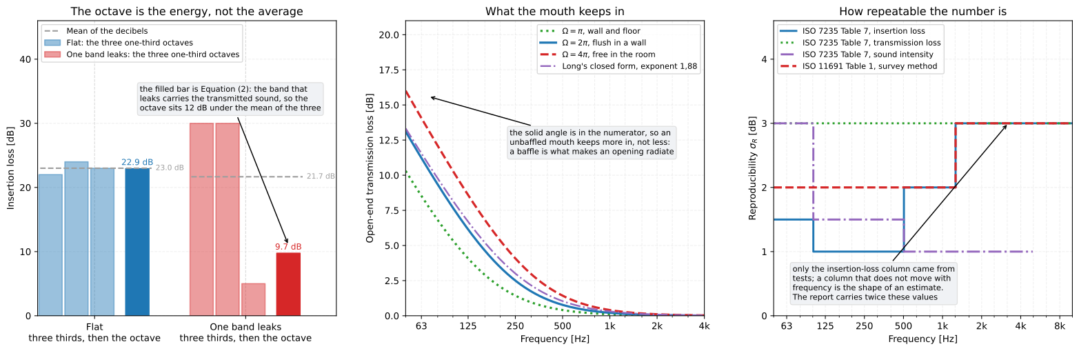
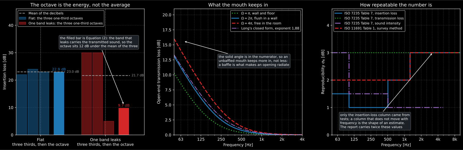
The three things a measurement report carries beyond the numbers themselves: how its octaves were folded, what its duct mouth was keeping in, and how far any of it can be trusted.

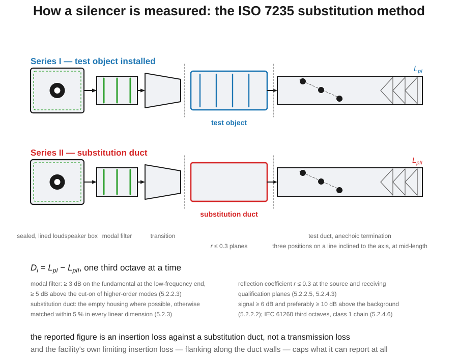
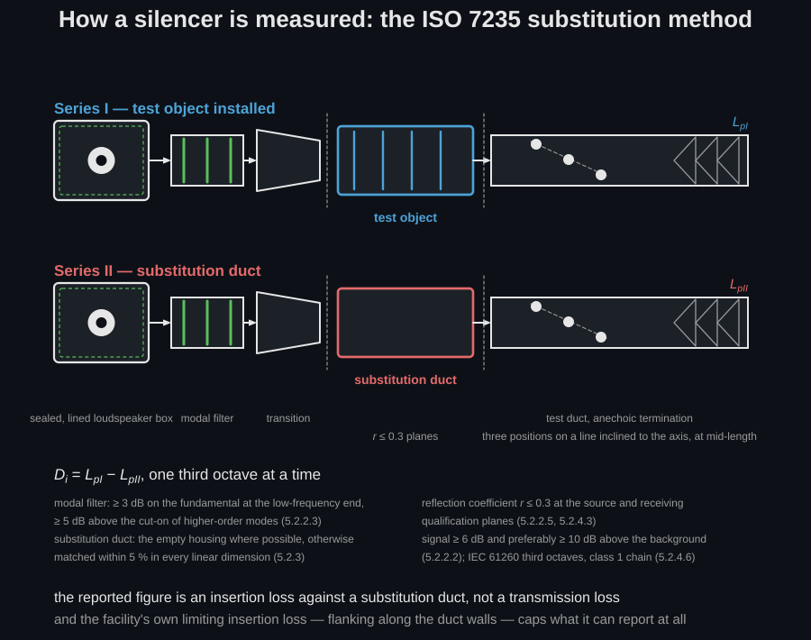
The two series are the whole method: everything else in both standards is about making sure nothing but the test object changed between them.

The measurement is the same in both:

with $\mathrm{I}$ the series that had the test object and $\mathrm{II}$ the series that had the substitution duct. ISO 11691 writes the identical thing as $D=L_{p1}-L_{p2}$, and numbers the two series the other way round: its 1 is the substitution duct. Two standards for one measurement, with opposite subscripts, is exactly the sort of thing that gets entered backwards, so the arguments here are named for what was in the duct rather than for either numbering.

from phonometry import noise_control

substitution = [88.0, 90.0, 91.0, 92.0, 92.0, 91.0]   # dB, empty duct
with_silencer = [84.0, 83.0, 79.0, 72.0, 66.0, 63.0]  # dB, silencer fitted

d_i = noise_control.substitution_insertion_loss(substitution, with_silencer)
print(d_i)                        # [ 4.  7. 12. 20. 26. 28.] dB

If the receiving room’s absorption moved between the two series, that difference is not yet the insertion loss. Clause 6.3 puts it right with $10\lg (T_2/T_1)$, where $T_2$ is the reverberation time measured with the test object installed. A room that got deader while the silencer was in it was flattering the silencer, and the correction takes that back:

corrected = noise_control.substitution_insertion_loss(
    substitution, with_silencer, reverberation_times=(2.1, 1.8),
)
print(corrected.round(2))         # [ 3.33  6.33 11.33 19.33 25.33 27.33] dB

Clause 6.3 also allows $T_2=T_1$ outright when the test object sits outside the room, and then the pair can be left out.

It is not a transmission loss. It is measured against a particular substitution duct in a particular rig, and it carries that rig with it in two ways worth naming.

The first is the limiting insertion loss: sound flanks along the duct walls rather than through the silencer, and no arrangement can measure past what its own flanking lets round. ISO 7235 has the laboratory measure that ceiling with the substitution duct acoustically blocked and record it as a function of frequency (7.4). A very large catalogue figure is a claim about the test arrangement as much as about the device.

The second is the receiving side, which decides how much of the sound the microphones see at all. ISO 7235 allows three (5.2.4): a reverberation room to ISO 3741 qualified at least down to the 125 Hz one-third octave, which is preferred; a test duct with an anechoic termination whose reflection coefficient is no greater than 0,3; or essentially free-field conditions at the open end. ISO 11691 keeps only the reverberation room and the free-field alternatives, and asks for 3,5 m of duct on each side of the silencer.

None of that is arithmetic, which is why the rest of this page is short. The arithmetic that remains is the part a reader can get wrong on paper.

A measurement is made in one-third octaves and often reported in octaves. ISO 11691 Equation (2) says how, and it is not an average of the three numbers:

The average is taken on what the silencer lets through. That matters because a silencer is rarely flat across an octave, and the band that leaks decides the answer:

thirds = [4.0, 7.0, 12.0, 20.0, 26.0, 28.0]
print(noise_control.octave_insertion_loss(thirds).round(2))
#                                 # [ 6.57 23.28] dB

The plain arithmetic means of the same two groups are 7,67 and 24,67 dB, so reading the decibels rather than the energy would have overstated both octaves by about a decibel. On a steeper silencer the gap is larger: three thirds of 30, 30 and 5 dB give 9,7 dB over the octave, not 21,7. Almost all the transmitted sound is coming through the one band that does not work, and Equation (2) is written out rather than described precisely so that this cannot be got wrong.

ISO 11691 states the assumption it rests on: the sound pressure levels of the three one-third octaves are taken to be equal in the series run with the substitution duct, which is what lets their energies be weighted equally.

In a test duct the spatial average comes from at least three microphone positions equally spaced on a line across the duct, spanning at least a quarter wavelength of the band, about half way along the duct. Three is enough only if the three agree. ISO 7235 Table 6 says how closely, and if the highest and lowest differ by more than that, five positions shall be used:

levels = [70.0, 74.0, 79.0]       # dB at the three key positions
print(noise_control.microphone_spread_limit(125.0))     # 7.0 dB
print(noise_control.microphone_positions_required(levels, 50.0))    # 3
print(noise_control.microphone_positions_required(levels, 125.0))   # 5

The same three levels are acceptable at 50 Hz, where the limit is 10 dB, and not at 125 Hz, where it is 7. The limit falls with frequency because a duct at low frequency has a standing-wave pattern that three points sample badly, and at high frequency does not.

One thing to know about Table 6: its rows read 50, 63, 80, 100, 125 and then > 160 Hz, so the 160 Hz one-third octave belongs to no row and is given no limit at all. Every other row names a single band, and 160 Hz is a one-third-octave centre like the rest, so it is read here as belonging to the last row. The gap is in the errata register.

Both standards answer, and neither answer is flattering.

ISO 11691 says outright that exact information on the precision of its method cannot be given, that interlaboratory tests would be needed for a real reproducibility standard deviation, and that this is what makes it a survey standard. Its Table 1 offers an estimate only: 2 dB up to the 1,25 kHz one-third octave and 3 dB above it.

ISO 7235 Table 7 has three columns, and the disagreement between them is the useful part:

for band in (50.0, 250.0, 1000.0, 4000.0):
    print(band, [
        noise_control.measurement_reproducibility(band, quantity=q)
        for q in ("insertion_loss", "transmission_loss", "intensity")
    ])
# 50.0   [1.5, 3.0, 3.0]
# 250.0  [1.0, 3.0, 1.5]
# 1000.0 [2.0, 3.0, 1.0]
# 4000.0 [3.0, 3.0, 1.0]

Insertion loss is measured best in the middle of the range and worst at the top; the sound-intensity route runs the other way; transmission loss is a flat 3 dB everywhere. Clause 7.9 explains why: only the insertion-loss column came from tests, on 1 m long parallel-baffle silencers, and the other two rest on experience. A column that does not move with frequency is the shape of an estimate, not of a measurement.

What goes on the report is twice the table value, for a coverage probability of 95 %:

print(noise_control.measurement_expanded_uncertainty(250.0))    # 2.0 dB
print(noise_control.measurement_expanded_uncertainty(4000.0))   # 6.0 dB

A silencer quoted at 25 dB in the 4 kHz band is being quoted to within 6 dB.

The survey method is deliberately narrow, and its limits are published rather than implied. The design velocity may not exceed 15 m/s, because the method runs the rig with no flow at all and so includes none of the self-generated noise. It is written for circular silencers from 80 mm to 2 m in diameter, or rectangular ones of comparable area. And the test ducts have to be close in cross section to what they feed, between 0,6 and 1,7 times the area of the silencer or the substitution duct (4.5). Outside that, the joints reflect more than the method allows for, and the library says so:

print(noise_control.substitution_area_ratio(0.0962, 0.0962))    # 1.0
print(noise_control.SURVEY_MAX_VELOCITY_M_S)                    # 15.0
print(noise_control.SURVEY_AREA_RATIO_RANGE)                    # (0.6, 1.7)

A duct radiating into a room does not hand the room everything that reaches its mouth. Well below the frequency at which the mouth is a wavelength across it is a poor radiator, and most of the energy turns round and travels back up the duct. Annex B.3 puts a number on it:

The group $4\pi f\sqrt{S}/c$ is the mouth measured in wavelengths, and $\Omega$ is the solid angle it radiates into. A 350 mm duct flush with a wall holds back 11 dB at 63 Hz and 0,05 dB at 2 kHz, which is nothing:

import numpy as np

bands = np.array([63.0, 125.0, 250.0, 500.0, 1000.0, 2000.0])
area = 0.0962                     # m2, a 350 mm circular duct

d_td = noise_control.open_end_transmission_loss(bands, area)
print(d_td.round(2))              # [11.23  6.14  2.5   0.77  0.21  0.05] dB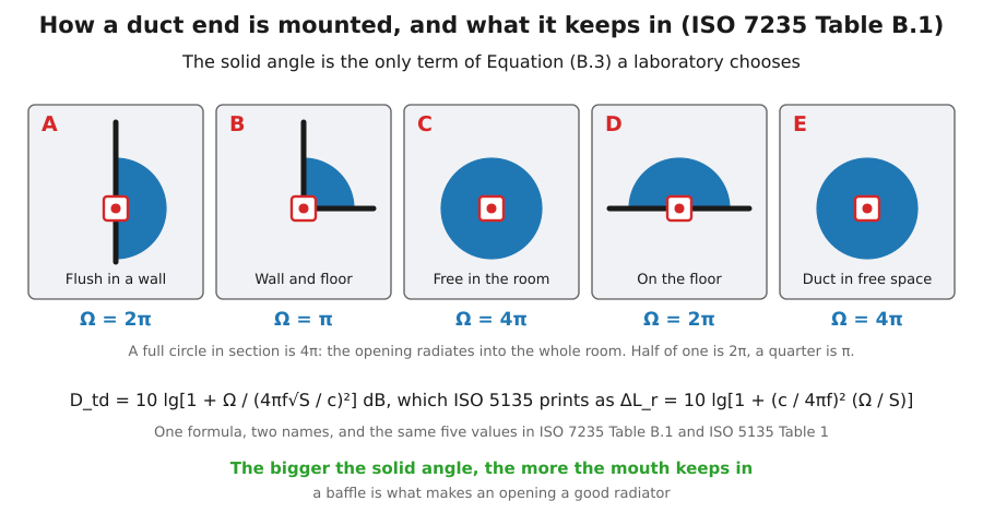

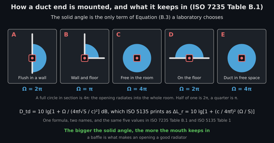
The solid angle is the only term of Equation (B.3) a laboratory chooses rather than measures, and the five choices are the same in both standards.

The solid angle is Table B.1, and the same five values are Table 1 of ISO 5135. It works the way round that surprises people: $\Omega$ sits in the numerator, so a duct ending in the middle of the room keeps more sound in than one flush with a wall, not less. A baffle is what makes an opening a good radiator, because it stops the pressure relieving round the rim of the mouth, and an unbaffled end of the same size sends more of the sound back up the duct:

free = noise_control.open_end_transmission_loss(
    bands, area, solid_angle_sr=noise_control.RADIATION_SOLID_ANGLES["C"],
)
print(free.round(2))              # [14.07  8.59  4.08  1.43  0.4   0.1 ] dB

Three more decibels at 63 Hz, and the reflection coefficient rises with it.

Both carriers are below the 857 Hz cut-on of a duct that wide, so the field inside it is the plane wave the whole of ISO 7235’s duct arithmetic assumes. The reflection coefficients read off the standing wave are the simulated geometry’s own, and not Equation (B.4): that closed form is a piston approximation for a circular mouth, where this is a slit in a screen. What the two share is the mechanism, and it is the mechanism that decides whether a level measured in a room is the level in the duct behind it.

Equation (B.4) says the same fact the other way round, as a pressure reflection coefficient, and the two close exactly on the energy: $D_{\mathrm{td}}=-10\lg (1-r^2)$ at every frequency, area and solid angle. That identity is the conformance anchor for both, because neither is printed with a worked value. It also has a use of its own: 5.2.4 qualifies a test duct as anechoic only below $r=0,3$, which this bare open end reaches somewhere between 500 Hz and 1 kHz.

r = noise_control.open_end_reflection_coefficient(bands, area)
print(r.round(3))                 # [0.962 0.87  0.662 0.404 0.215 0.11 ]

The library carries a second closed form for the same physics, Reynolds’ as given by Long, in end_reflection_loss_closed_form. It raises the same argument to 1,88 rather than to 2, and for a circular duct in free space the two read $10\lg [1+(c/\pi fd{)}^2]$ against $10\lg [1+(c/\pi fd{)}^{1,88}]$. They agree closely where the argument is near 1 and part company at the ends of the range.

Two quantities need it. Equation (6) turns the measured insertion loss of an air-terminal unit into its transmission loss by putting back what the mouth was keeping in anyway, so the two are the same number at the top of the range and eleven decibels apart at the bottom:

d_i = np.array([4.0, 7.0, 12.0, 20.0, 26.0, 28.0])
print(noise_control.measured_transmission_loss(d_i, d_td).round(2))
#                                 # [15.23 13.14 14.5  20.77 26.21 28.05] dB

And Equation (7) makes the flow noise a sound power, $L_W=\overline{L_p}+D_{\mathrm{td}}+C$, where $C$ is the ISO 3741 level difference between the power radiated into the room and the average pressure in it. Clause 6.4 is explicit that $\overline{L_p}$ goes in without a background correction: the two series are reported separately and the reader subtracts them.

The modal filter between the source and the test object exists to stop higher-order modes reaching the silencer, and its requirement steps at the frequency where those modes can propagate in the connected ducts: at least 3 dB of longitudinal attenuation of the fundamental at the low-frequency end, and at least 5 dB above that frequency (5.2.2.3). NOTE 2 prints where it is:

print(round(noise_control.modal_filter_cut_on(diameter_m=0.4), 1))          # 505.9 Hz
print(round(noise_control.modal_filter_cut_on(larger_dimension=0.5), 1))  # 343.0 Hz

The rectangular form, $0,5c/H$, is exact: the first mode of a rigid rectangular duct is a half wavelength across the larger dimension. The circular one, $0,59c/d$, is rounded. The exact coefficient is the first zero of $J_1^{\prime }$ over $\pi$, which is 0,58607, so Equation (4) sits 0,67 % high: on the 0,4 m duct of the ISO 11691 sound source that is 505,9 Hz where circular_duct_cut_on gives 502,6 Hz. Three and a half hertz does not matter for choosing a modal filter, and it is worth knowing which of the two numbers is the physics.

The third thing ISO 7235 measures has nothing to do with sound. A silencer that works and costs a fan half its pressure is not a good silencer, so 6.5 measures the total pressure loss coefficient, and the whole point of the coefficient rather than the loss is that a loss means nothing without the flow it was measured at.

Start with the air. Equation (10) is the ideal gas law with the standard’s own constants, and the static pressure it takes is a gauge pressure against the ambient, so the two add:

rho = noise_control.normal_air_density(200.0, 101325.0, 20.0)
print(round(rho, 4))              # 1.2073 kg/m3

q_v = noise_control.volume_flow_rate(1.2, rho)
print(round(q_v, 4))              # 0.9939 m3/s

ISO 7235 prints $R=287$ and writes the absolute temperature as $\theta +273{}^{\circ }\text{C}$, neither of which is the accurate figure. The offset alone puts the density 0,051 % high at 20 °C, and the gas constant adds 0,017 % to that, for 0,069 % in all. It does not cancel: the same density is in the dynamic pressure of both test series, so the coefficient is scaled by that one factor rather than shifted, and comes out 0,069 % low. That is far under the uncertainty of a pressure-loss test, and using the printed constants is what reproduces a result computed to the standard, so the library keeps both. It is recorded in the errata register as a property of the source rather than as a defect.

Equation (9) rather than (8) is used when the flow meter and the test object are far enough apart in temperature or pressure that their density ratio leaves 0,98 to 1,02: outside that window the meter is not measuring the flow the test object sees.

The velocity head is Equation (13), and the coefficient is the loss divided by it:

p_d1 = noise_control.dynamic_pressure(q_v, 0.0962, rho)
print(round(p_d1, 2))             # 64.44 Pa

delta_p_t = noise_control.total_pressure_loss(45.0, p_d1, 0.0962, 0.0962)
print(round(noise_control.pressure_loss_coefficient(delta_p_t, p_d1), 3))
#                                 # 0.698

That number belongs to the object rather than to the test point, at least to the extent the flow is dynamically similar: a loss grows as the square of the velocity and so does the head it is divided by, so the algebra returns the same coefficient at twice the flow. Real flow is not exactly similar, because doubling the rate doubles the Reynolds number too, and that is the reason 6.5.2 measures at five rates and averages rather than trusting one. The drift over a test range is small, and it is not zero.

Equation (12) is the part worth reading twice. Measuring static pressures on both sides is not enough when the two sides are different sizes, because an object that widens the duct converts velocity head back into static pressure and a static difference alone would credit it with a recovery that is only bookkeeping. The bracket $1-(S_1/S_2{)}^2$ puts it back, and the NOTE to Equation (14) says what usually happens to it: as a rule $S_1=S_2$, and it vanishes. Where it does not, it is not small:

widening = noise_control.total_pressure_loss(45.0, p_d1, 0.0962, 2 * 0.0962)
print(round(noise_control.pressure_loss_coefficient(widening, p_d1), 3))
#                                 # 1.448, from the same 45 Pa of static loss

The fundamental method of 6.5.2.2 measures the coefficient the way the acoustic half measures insertion loss: run the rig with the test object, run it again with the substitution duct, and the difference belongs to the object. The computational route of 6.5.2.2.3 does the subtraction on the coefficients rather than on the pressures, which means the two series need share neither their flow rates nor even their number of points:

import numpy as np

heads = np.array([20.0, 40.0, 60.0, 80.0, 100.0])   # Pa, five airflow rates
with_object = 2.5 * heads
without = 0.6 * heads

zeta = noise_control.average_pressure_loss_coefficient(
    with_object, heads, without, heads,
)
print(round(zeta, 3))             # 1.9

Five rates per series, spread evenly over the range, and the lowest has to produce more than 10 Pa so that the smallest number in the average is still a measurement rather than the resolution of the manometer. The library says so on both counts: average_pressure_loss_coefficient warns below five points, and pressure_loss_coefficient warns on a loss of 10 Pa or less, the boundary included, because the clause reads greater than.

What the flow has to be before any of that counts is a matter of geometry. The upstream duct is straight for five equivalent diameters or two metres, whichever is greater, so that the velocity profile has settled; it must be uniform to ±10 % of the mean over the section, excluding the 15 mm nearest the walls, surveyed ten points along each of two perpendicular axes about $1,5d_e$ upstream. The two length rules cross at a 0,4 m equivalent diameter:

print(round(noise_control.upstream_straight_length(0.0962), 2))   # 2.0 m
print(round(noise_control.upstream_straight_length(0.5), 2))      # 3.99 m

ISO 5135:1999 measures something else again: the sound power an air-terminal device, air-terminal unit, damper or valve radiates, determined in a reverberation room to ISO 3741. What a designer needs is not that but what the device puts into the duct behind it, and Equation (1) is the step between them:

The correction $\Delta L_{\mathrm{r}}$ is Equation (2) of ISO 5135, and it is worth writing both printings side by side:

Expand either and both become $10\lg [1+\Omega c^2/(16{\pi }^2{f}^{2}S)]$. They are one formula, their two solid-angle tables agree entry for entry, and open_end_transmission_loss is both. That is why nothing new appears here for the correction itself:

d_lr = noise_control.open_end_transmission_loss(bands, area)
lw_room = np.array([58.0, 60.0, 61.0, 59.0, 55.0, 50.0])
print(noise_control.duct_sound_power_level(lw_room, d_lr).round(2))
#                                 # [69.23 66.14 63.5  59.77 55.21 50.05] dB

A device measured in a room is understated in the duct by eleven decibels at the bottom of the range and by nothing at the top. The NOTE to Table 1 offers a way round the correction rather than a second formula for it: fit a transmission element to ISO 7235 and no correction is applied at all.

A device is not tested at the one operating point a designer will use it at. ISO 5135 5.5.2 fits a straight line by least squares through the levels against $\lg q_V$ when the tests were made at a constant pressure loss coefficient, or against $\lg \Delta p_{\mathrm{t}}$ when they were made at a constant flow rate. The same fit serves the band levels and the A-weighted one:

duty = np.array([0.05, 0.1, 0.2, 0.4, 0.8])          # m3/s
levels = np.array([38.0, 44.5, 50.0, 56.5, 62.0])    # dB(A)

line = noise_control.fit_operating_line(duty, levels)
print(round(line.slope, 2))               # 19.93 dB per decade
print(round(line.maximum_deviation, 2))   # 0.3 dB
print(round(line.level_at(0.3), 1))       # 53.7 dB(A)

Two rules keep that honest, and the library says so on both rather than refusing: a fit that is not a straight line is still a fit, and a level read past the range is still a number, and what the standard asks is that a report be honest about them. The measured points have to sit within 3 dB of the line, because past that the levels are not a straight line in this variable and reading the line off means nothing. And the line may be extended down to half the smallest duty measured and up to twice the largest, and no further, which for these five points is 0.025 to 1.6 m³/s. Either one out of range raises a SilencerMeasurementWarning:

print(line.valid_range)           # (0.025, 1.6)

Clause 8 k) closes the loop: a report gives the fully corrected levels to the nearest half decibel and has to state which of them were extrapolated rather than measured directly. .plot() draws that distinction, shading the two ends of the range that are extrapolation.

• Covered

  The arithmetic of the substitution measurement: Equation (1) of both standards through substitution_insertion_loss, with the reverberation-time correction of ISO 7235 6.3; the octave fold of ISO 11691 Equation (2) through octave_insertion_loss; ISO 7235 Table 6 and the three-or-five rule of 6.2.1 through microphone_spread_limit and microphone_positions_required; the reproducibility of ISO 11691 Table 1 and of all three columns of ISO 7235 Table 7, with the expanded uncertainty of 7.9; and the scope ISO 11691 draws in 1.1 and 4.5, including the area-ratio check that warns outside it. The open end of the duct: Equations (B.3) and (B.4) through open_end_transmission_loss and open_end_reflection_coefficient, with the five solid angles of Table B.1; the transmission loss of Equation (6) and the flow-noise sound power of Equation (7); and the cut-on frequencies of Equations (4) and (5) that the modal-filter requirement of 5.2.2.3 steps at. And the flow half of 6.5: the gas law of Equations (10), (21) and (22), the volume flow rate of (8) and (9), the velocity head of (13), (16), (19) and (20), the total pressure of (11), the area-change correction of (12), the pressure loss coefficient of (14) and (17), the substitution average of (18), and the settling length of 6.5.2.2.1. From ISO 5135: the duct sound power level of Equation (1); Equation (2), which is Equation (B.3) of ISO 7235 written out again and is served by the same function; and the least-squares operating line of 5.5.2 through fit_operating_line, with the 3 dB limit on the fit, the half-to-twice range it may be read over, and a .plot() that shades the part of that range which is extrapolation.

• Not covered

  Nothing here builds a test facility or checks one: the modal-filter attenuation, the anechoic termination’s reflection coefficient, the substitution duct’s dimensional tolerance and the limiting insertion loss are described but not computed, and Equation (7) is given the room correction rather than deriving it. The flow measurement itself is not modelled: the differential-pressure devices of ISO 5167-1, the velocity survey and the piezometric ring are procedure rather than arithmetic. Nothing here builds a reverberation room or qualifies one: the ISO 3741 determination both standards hand their receiving side to is a separate page, and the background corrections, the discrete-tone check and the room qualification belong to it. ISO 11820, which measures a silencer in situ where the substitution trick is usually impossible, is not implemented at all. Neither is ISO 11820, which measures a silencer in situ, where the substitution trick is usually impossible.

References

Section titled “References”- International Organization for Standardization. (1995). Acoustics — Measurement of insertion loss of ducted silencers without flow — Laboratory survey method (ISO 11691:1995). The survey-grade sibling: its Equations (1) and (2), Table 1, and the scope it draws in 1.1 and 4.5. Read from BS EN ISO 11691:2009, which endorses it without modification.
- International Organization for Standardization. (2003). Acoustics — Laboratory measurement procedures for ducted silencers and air-terminal units — Insertion loss, flow noise and total pressure loss (ISO 7235:2003). The measurement itself: Equation (1), the reverberation correction of 6.3, Table 6 and the rule of 6.2.1, and Table 7 with the coverage factor of 7.9. Read from BS EN ISO 7235:2009, which endorses it without modification.
- International Organization for Standardization. (2010). Acoustics — Determination of sound power levels of noise sources using sound pressure — Precision methods for reverberation test rooms (ISO 3741:2010). The sound power determination both standards hand the receiving side to, and the source of the reverberation times the correction of 6.3 needs.