Silencers
Standards: ISO 7235Key references: Bies et al. 2017Munjal 2014Vér & Beranek 2006
A silencer earns its keep in a duct: between an engine and its tailpipe, between a fan and the room it serves. Two working principles divide the field. A reactive silencer attenuates by reflecting sound with impedance discontinuities (chambers, side branches) and dominates at low frequency, where a tone from a firing engine or a fan blade passage can be targeted exactly; a dissipative silencer absorbs sound in a porous lining and dominates broadband, at mid and high frequency. This guide covers the reactive family phonometry implements with the engineering theory of Bies, Hansen & Howard and Munjal’s transfer-matrix formulation: the four-pole method, the closed-form expansion chamber, the Helmholtz, quarter-wave and extended-tube resonators, the independent FDTD cross-check, and the design trade-offs against dissipative linings. The rest of the installation, HVAC duct attenuation, flow noise and machine enclosures, lives in Industrial noise control.
1. Reactive silencers (four-pole method)
Section titled “1. Reactive silencers (four-pole method)”Reflection is computed one element at a time. Each acoustic element is a 2x2 transfer matrix relating the pressure and volume velocity at its two ends, and a compound silencer is the ordered matrix product of its elements (Bies §8.9). A straight duct of length and area is
and a side branch of impedance is the shunt
. The
transmission loss follows from the compound matrix with the port
impedances and
(Munjal Eq. (3.27); Bies Eq. (8.141) prints the T11/T22 impedance
weights of this formula inverted and fails the sudden-expansion limit, see the
errata registry)
which for equal inlet/outlet areas reduces to (Bies Eq. (8.148))
and the insertion loss for a source impedance and radiation impedance is the extra attenuation over a direct connection.
Expansion chamber
Section titled “Expansion chamber”The simplest silencer, a chamber of area and length between pipes of area , has the closed-form transmission loss (Bies Eq. (8.111)) with area ratio
peaking at when and dropping to at where the chamber is a half-wavelength long and transparent. The four-pole product reproduces this exactly.
import numpy as npfrom phonometry import noise_control
freqs = np.linspace(20.0, 2000.0, 2000)res = noise_control.expansion_chamber(freqs, length=0.3, chamber_area=0.04, pipe_area=0.01)print(round(res.transmission_loss.max(), 2))   # 6.55 dB peak (m = 4)# The troughs at f = n c / 2L are exactly 0 dB (no dissipation).print(round(float(res.transmission_loss[np.argmin(res.transmission_loss)]), 6))
The one-liner res.plot() draws the transmission loss of the chamber (and its
insertion loss when the source and radiation impedances are given). The figure
below sweeps the area ratio instead: a larger mismatch lifts every peak,
but the troughs stay at 0 dB and the peaks stay at the same frequencies, set
only by the chamber length.
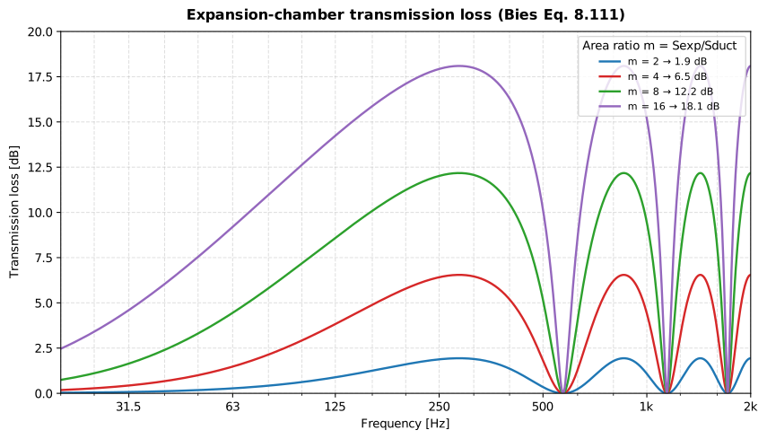
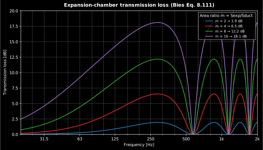
Two design levers, and only one of them is cheap. The peak, , grows only as the logarithm of the area ratio: buys 1.9 dB and buys 18.1 dB, so quadrupling the chamber cross-section is worth about 6 dB, while the trough frequencies never move at all, because they depend on the length alone. A chamber is lengthened to move the notch and widened to deepen the peak.
Show the code for this figure
import matplotlib.pyplot as pltimport numpy as npfrom phonometry import noise_control
freqs = np.linspace(20.0, 2000.0, 2000)
# One line for one chamber: TL vs frequency, plus the insertion loss when the# two acoustic impedances are given (Pa.s/m3 -- see the next subsection for# where they come from). With both set to rho c / S = 4.14e4 for this 0.01 m2# pipe the two curves coincide, which is what "anechoic ports" means.noise_control.expansion_chamber(freqs, 0.3, 0.04, 0.01,                                source_impedance=4.14e4, radiation_impedance=4.14e4).plot()plt.show()
# By hand: the family of area ratios of the concept figure.fig, ax = plt.subplots()for m in (2.0, 4.0, 8.0, 16.0):    res = noise_control.expansion_chamber(freqs, 0.3, m * 0.01, 0.01)    ax.plot(freqs, res.transmission_loss, label=f"m = {int(m)}")ax.set_xlabel("Frequency [Hz]"); ax.set_ylabel("Transmission loss [dB]")ax.legend()plt.show()
The numbers passed to expansion_chamber describe a real device, and
.plot_geometry() draws it: the same 0.3 m chamber with its 4:1 area ratio,
to scale and fully dimensioned.
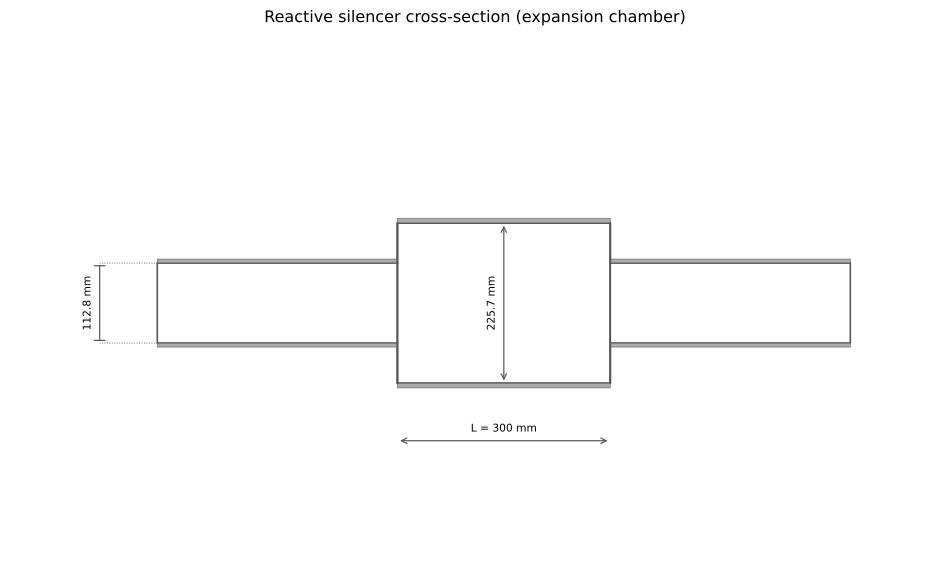
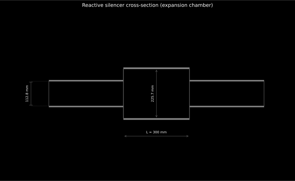
The chamber behind the curves above, to scale: the areas enter the four-pole method only through the ratio , and the drawing uses the equivalent circular diameters of the 0.04 and 0.01 m² cross-sections.
Show the code for this figure
import matplotlib.pyplot as pltimport numpy as npfrom phonometry import noise_control
freqs = np.linspace(20.0, 2000.0, 2000)res = noise_control.expansion_chamber(freqs, length=0.3, chamber_area=0.04, pipe_area=0.01)
# One line: the dimensioned cross-section of the chamber just computed.res.plot_geometry()plt.show()
# The same drawing without a result, from the free function:noise_control.plot_silencer_geometry("expansion chamber", length=0.3,                                     chamber_area=0.04, pipe_area=0.01)plt.show()
Transmission loss, insertion loss, and which one a datasheet quotes
Section titled “Transmission loss, insertion loss, and which one a datasheet quotes”Three quantities are in circulation and they are not interchangeable. Transmission loss compares the incident power entering the element with the power leaving it into a reflection-free termination, so it is a property of the element alone, which is exactly why it can be computed from geometry, and why the formula above sets and without asking what the silencer is connected to. Insertion loss compares the level at a fixed point with and without the element in place, so it depends on the source and on what the duct radiates into, and the same chamber shows a different insertion loss in two installations. Noise reduction is the plain level difference across the element, which is what a two-microphone measurement in a live duct returns.
A reactive element is where they diverge most, because it works by sending
energy back towards a source that may re-reflect it. Both impedances are
acoustic, in Pa·s/m³ (pressure per volume velocity), and they have a scale:
for the 0.01 m² inlet pipe is , so a source far
above that approximates a constant-volume-velocity machine such as a
reciprocating engine and one far below it a constant-pressure source. The
termination is not a free choice at all; for a duct discharging into a room it
is the radiation impedance of the open end,
, whose normalised and the
radiating piston
of the electroacoustics domain returns as radiating_piston(...).resistance and
.reactance (its radiation_resistance and radiation_reactance are the
mechanical impedance in N·s/m, a factor away,
and an easy thing to feed in by mistake). The source impedance of a fan or an
engine, by contrast, is rarely known and strongly frequency dependent, which is
precisely why insertion loss is a measured quantity in practice.
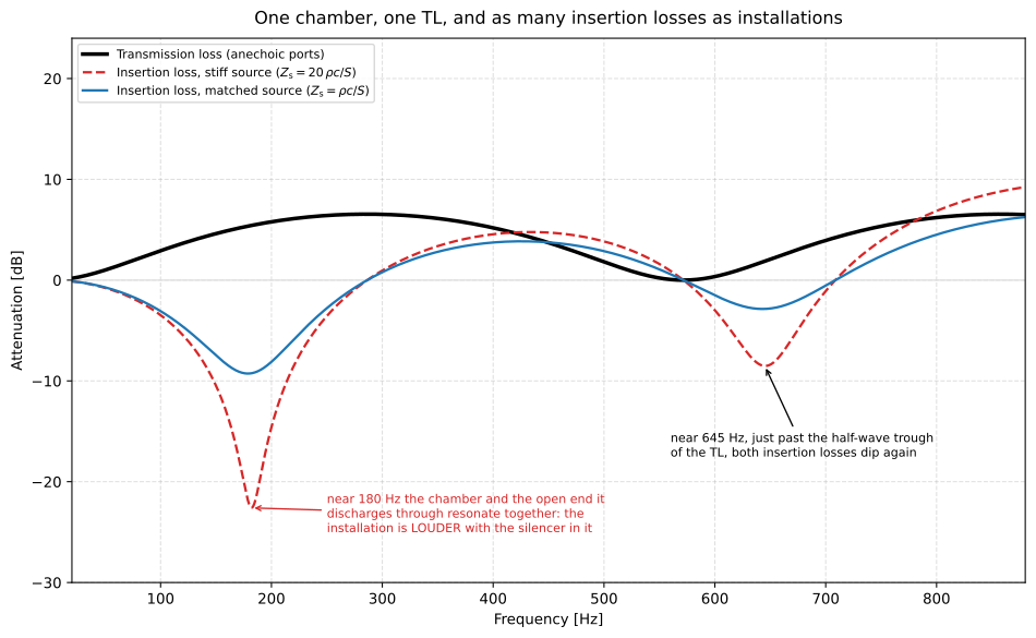
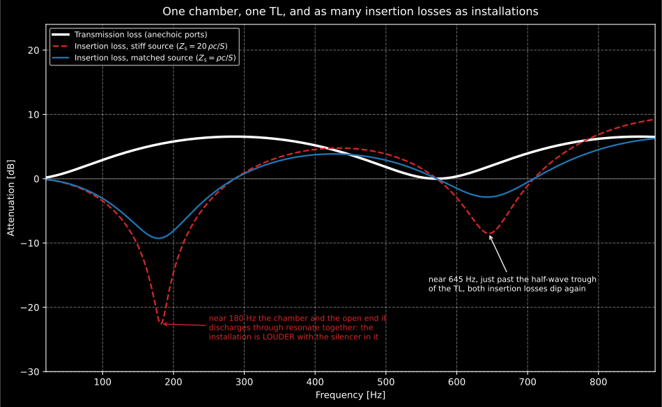
The same chamber, three answers. Transmission loss never goes below zero, because it is defined against a termination that reflects nothing. Insertion loss can: near 180 Hz this chamber and the open end it discharges through resonate together, and the installation is louder with the silencer in it than without: 9.3 dB louder for a source matched to the pipe and 22.6 dB for a stiff one, where the transmission loss reads a comfortable +5 dB. This is why a catalogue publishes a dynamic insertion loss measured with the design airflow in the design direction, and why a computed TL is a sizing tool rather than a specification.
Show the code for this figure
import matplotlib.pyplot as pltimport numpy as npfrom scipy import special          # expansion_chamber: imported in section 1
freqs = np.linspace(20.0, 880.0, 1600)     # below the 890.8 Hz cut-onrho, c, pipe_area = 1.206, 343.0, 0.01z0 = rho * c / pipe_area                   # 41.4 kPa.s/m3
# The open end, as the baffled piston: R1(2ka) and X1(2ka). The same two# numbers come out of radiating_piston(a, freqs).resistance / .reactance.a = np.sqrt(pipe_area / np.pi)x = 2.0 * (2.0 * np.pi * freqs / c) * az_r = z0 * ((1.0 - 2.0 * special.j1(x) / x)            + 1j * (2.0 * special.struve(1, x) / x))
# One line: the result draws the insertion loss beside the transmission loss# whenever both impedances are given.noise_control.expansion_chamber(freqs, 0.3, 0.04, pipe_area,                                source_impedance=z0, radiation_impedance=z_r).plot()plt.show()
# By hand: the two source impedances of the figure against the same outlet.fig, ax = plt.subplots()ax.plot(freqs, noise_control.expansion_chamber(freqs, 0.3, 0.04, pipe_area).transmission_loss,        label="Transmission loss")for factor, label in ((20.0, "stiff source"), (1.0, "matched source")):    res = noise_control.expansion_chamber(freqs, 0.3, 0.04, pipe_area,                                          source_impedance=factor * z0, radiation_impedance=z_r)    ax.plot(freqs, res.insertion_loss, label=f"Insertion loss, {label}")ax.set_xlabel("Frequency [Hz]"); ax.set_ylabel("Attenuation [dB]")ax.legend()plt.show()
The rule that follows is short: do not compare a computed transmission loss with a published insertion loss. Write requirements against insertion loss with the termination stated, get the number from the supplier or from a test (section 3), and treat the transmission loss this page computes as the tool that tells you which geometry to ask for.
The clip below runs an chamber of the same 0.30 m length in a 2D FDTD duct at its two characteristic frequencies. At the chamber is a half-wave resonator and the tone crosses as if it were not there; at the two area jumps reflect in phase and send the wave back up the inlet, the 6.5 dB peak of the four-pole curve above.
A 2D FDTD duct with a 0.30 m expansion chamber of area ratio 4, drawn as hardware between a loudspeaker and an anechoic termination, at two frequencies side by side. At 572 Hz the pressure envelope stays flat and the tone crosses the chamber unchanged with the annotated transmission loss of 0.0 dB; at 286 Hz a standing wave fills the inlet pipe and the outlet is left with less than half the amplitude, matching the annotated 6.5 dB peak.
A 2D FDTD duct with a 0.30 m expansion chamber of area ratio 4, drawn as hardware between a loudspeaker and an anechoic termination, at two frequencies side by side. At 572 Hz the pressure envelope stays flat and the tone crosses the chamber unchanged with the annotated transmission loss of 0.0 dB; at 286 Hz a standing wave fills the inlet pipe and the outlet is left with less than half the amplitude, matching the annotated 6.5 dB peak.
Side-branch and extended-tube resonators
Section titled “Side-branch and extended-tube resonators”A Helmholtz resonator (neck area , effective length , cavity volume ) and a closed quarter-wave tube (length ) each short the duct at their tuning frequency, giving a sharp transmission-loss spike there: (Bies Eq. (8.46)) and (Eq. (8.44)). An extended-tube chamber buries quarter-wave side branches in an expansion chamber to fill the plain chamber’s troughs.
Both lengths are effective lengths, and both functions take them that way
(neck_length and length are documented as , end corrections included).
The air in a neck does not stop moving at the mouth: it drags a slug of air
along on each side, so the mass that resonates against the cavity belongs to a
tube longer than the one that was drilled. Add about per flanged end
and about per free end, for a neck of radius , at both ends of a
Helmholtz neck and at the open (duct) end only of a quarter-wave stub. The
resonator drawn below is the case in point: its neck is 11.3 mm across
( mm) and 20 mm long, so mm and the tuning falls from the 122.1 Hz the drilled length returns to
100.3 Hz, a 22 % error on a notch the figure below shows to be only a few
hertz wide. The shorter and wider the neck, the larger the correction in
relative terms, which is exactly the regime a compact resonator lives in, so
the practical procedure is to compute a nominal length, build it long, and
trim it against a measurement.
import numpy as npfrom phonometry import noise_control
f = np.linspace(20.0, 600.0, 4000)
hr = noise_control.helmholtz_resonator(f, duct_area=0.01, neck_area=1e-4,                                       neck_length=0.02, cavity_volume=1e-3)print(round(float(hr.resonances[0]), 1))       # 122.1 Hz, for le = 20 mmhr.plot()   # TL spike at the tuning frequency (needs matplotlib)
qw = noise_control.quarter_wave_resonator(f, duct_area=0.01, length=0.3, branch_area=2e-3)print(round(float(qw.resonances[0]), 1))       # 285.8 Hz = c / 4 le
# Bies Example 8.1, the published anchor: a 1.516 m stub at c = 343.24 m/s.print(round(float(noise_control.quarter_wave_resonator(    f, duct_area=0.01, length=1.516, branch_area=2e-3,    speed_of_sound=343.24).resonances[0]), 1))  # 56.6 Hz
# The same stub in hot exhaust gas: c(500 degC) = 343*sqrt(773/293) = 557 m/s# (see the caution below), which moves the notch by a factor 1.62.f_hot = np.linspace(20.0, 900.0, 6000)qw_hot = noise_control.quarter_wave_resonator(f_hot, duct_area=0.01, length=0.3,                                              branch_area=2e-3, speed_of_sound=557.0)print(round(float(qw_hot.resonances[0]), 1))   # 464.2 Hz, not 285.8
# Each extension is a quarter-wave stub, so its own length picks the trough# it fills: L/4 = 0.1 m shorts the duct at c/4(L/4) = c/L, the chamber's# second trough, and L/2 = 0.2 m would take the first one at c/2L.et = noise_control.extended_tube_chamber(f, length=0.4, chamber_area=0.04, pipe_area=0.01,                                         inlet_extension=0.1)print(round(float(et.transmission_loss[np.argmin(abs(f - 428.75))]), 1))# 0.6 dB at c/2L: the L/4 stub is tuned an octave above it
An extension is a quarter-wave stub buried inside the chamber, so its own length decides which trough it fills: a stub of length shorts the duct at . The plain 0.4 m chamber is transparent at Hz and again at Hz. The 0.1 m inlet extension () is tuned to 858 Hz, so it shorts the second trough and leaves the first almost untouched at 0.6 dB; the 0.2 m outlet extension () is the one tuned to 429 Hz, and the pair covers both. The trade is visible in the same figure: on its own the inlet extension does not remove the trough it misses, it moves it, to 444 Hz.
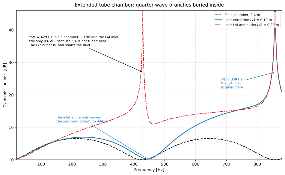
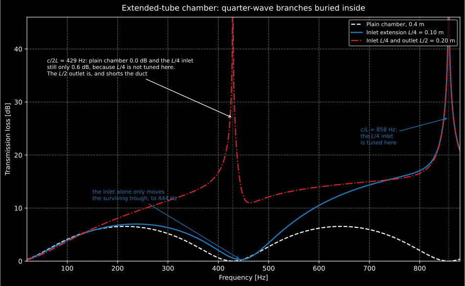
What an internal extension buys, and what it costs. The plain chamber’s 0 dB troughs at every half wavelength are its fatal defect, and each extension shorts exactly the one its own length tunes: takes the first, the second. A single extension therefore moves the trough it misses rather than removing it, which is why the extensions are sized in pairs and why an extended-tube chamber is designed against the source spectrum rather than in general.
Show the code for this figure
import matplotlib.pyplot as plt
# `f`, and extended_tube_chamber / expansion_chamber, as in section 1.plain = noise_control.expansion_chamber(f, 0.4, 0.04, 0.01)inlet = noise_control.extended_tube_chamber(f, 0.4, 0.04, 0.01, inlet_extension=0.1)both = noise_control.extended_tube_chamber(f, 0.4, 0.04, 0.01, inlet_extension=0.1,                                           outlet_extension=0.2)
# One line for one device:inlet.plot()plt.show()
fig, ax = plt.subplots()for res, label in ((plain, "Plain chamber"), (inlet, "Inlet L/4"),                   (both, "Inlet L/4 and outlet L/2")):    ax.plot(f, res.transmission_loss, label=label)ax.set_xlabel("Frequency [Hz]"); ax.set_ylabel("Transmission loss [dB]")ax.set_ylim(0.0, 46.0)ax.legend()plt.show()
The extension is a real piece of pipe pushed into the chamber, and
.plot_geometry() draws it to scale like every other device on this page.
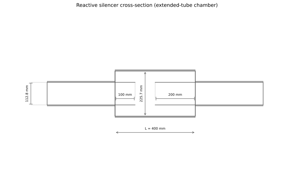
The same 0.4 m chamber as above, with the inlet tube pushed 100 mm in and the outlet 200 mm. Nothing is added on the outside: the two quarter-wave branches are the annular spaces the extensions create.
Show the code for this figure
import matplotlib.pyplot as plt
# One line: the dimensioned cross-section of the device just computed.noise_control.extended_tube_chamber(f, 0.4, 0.04, 0.01, inlet_extension=0.1,                                    outlet_extension=0.2).plot_geometry()plt.show()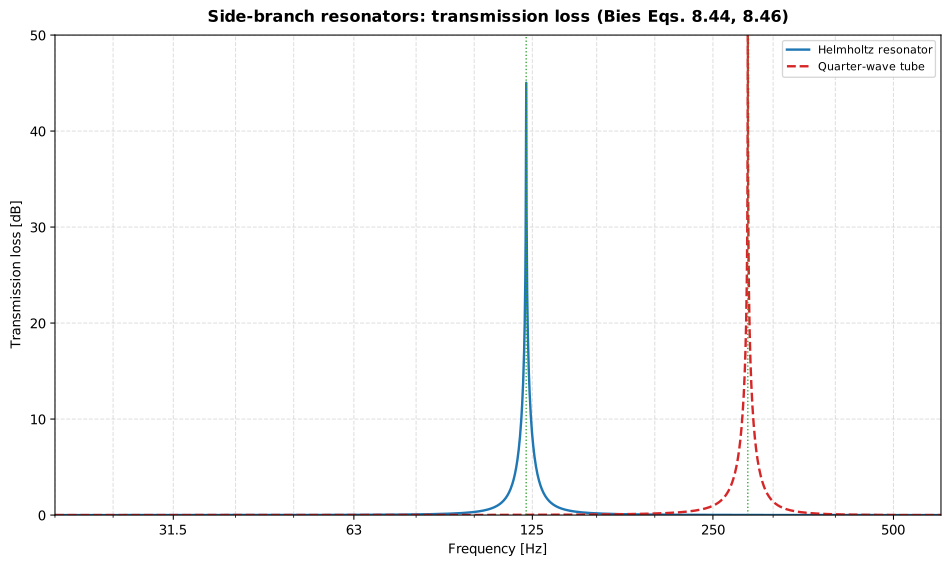
Each side branch shorts the duct at its own tuning frequency and is nearly transparent elsewhere: the narrow spike is why resonators are matched to a firing frequency or a fan blade-passing tone rather than used broadband.
Do not read the height of that spike. Both branch models default to
resistance=0.0, so the branch is a perfect short at and the computed
transmission loss diverges there; what the figure shows is where the frequency
grid happened to land, which is why the by-hand code below has to clamp the axis
at 50 dB. What limits the peak in metal is the viscous loss in the neck, the
radiation from the cavity walls and any damping deliberately added. A well-made
resonator delivers something like 15 to 25 dB at its tuning frequency, over a
relative bandwidth set by its and typically a few per cent, a fraction of
an octave. resistance= is where a measured or estimated acoustic resistance
goes, and adding it lowers and broadens the peak, which is the trade between
depth and tolerance to a tuning error. Read that beside the end-correction
warning above: a notch 22 % off its target is worth nothing, so the broader
damped design is usually the safer one.
Show the code for this figure
import matplotlib.pyplot as pltimport numpy as npfrom phonometry import noise_control
f = np.linspace(20.0, 600.0, 4000)hr = noise_control.helmholtz_resonator(f, duct_area=0.01, neck_area=1e-4,                                       neck_length=0.02, cavity_volume=1e-3)qw = noise_control.quarter_wave_resonator(f, duct_area=0.01, length=0.3, branch_area=2e-3)
# One line for one device: TL vs frequency with the resonance marked.hr.plot()plt.show()
# By hand: both side branches on the same axes.fig, ax = plt.subplots()ax.plot(f, hr.transmission_loss, label="Helmholtz resonator")ax.plot(f, qw.transmission_loss, "--", label="Quarter-wave tube")for fr in (hr.resonances[0], qw.resonances[0]):    ax.axvline(float(fr), ls=":", color="#2ca02c")ax.set_xlabel("Frequency [Hz]"); ax.set_ylabel("Transmission loss [dB]")ax.set_ylim(0.0, 50.0)ax.legend()plt.show()
Why is the notch only a few hertz wide at all? Because a resonator takes time to work, and the clip below shows it doing so, on this page’s own 0.30 m stub in a 2D FDTD duct. A side branch does not block the duct the instant the tone arrives: it has to charge. Driven at the tuning frequency, the pressure at the stub’s closed end ratchets up over about six periods to 8.2 times the incident wave (the lossless branch at exact resonance would reach ten, twice the duct-to-branch area ratio); driven at 150 Hz the same stub settles at 1.5 times within a couple of periods and never charges, which is the whole notch mechanism seen once; the charge has the percent-wide bandwidth , while the lossless TL spike is hertz-wide. The clip also runs the trim procedure of the end-correction warning above on screen: built at exactly the drilled 300 mm, the simulated device rings at 272.9 Hz rather than 285.8, an effective length mm, and it still charges fully because the 4.7 % detuning sits inside the 13 % charge bandwidth. No transmission loss is annotated anywhere on it: at the tuning frequency the lossless model’s TL is infinite, so a finite number there would only be restating the frequency grid.
A 2D FDTD duct carrying the guide's 0.30 m closed quarter-wave stub, driven at the 285.8 Hz tuning frequency and at 150 Hz side by side, with the closed-end pressure of both runs traced below. On tune the pressure inside the stub ratchets up over about six periods to 8.2 times the incident wave; off tune it settles at 1.5 times immediately and never charges. An annotation reports that the built 300 mm stub rings at 272.9 Hz, an effective length of 314 mm, so a built device would be trimmed to tune.
A 2D FDTD duct carrying the guide's 0.30 m closed quarter-wave stub, driven at the 285.8 Hz tuning frequency and at 150 Hz side by side, with the closed-end pressure of both runs traced below. On tune the pressure inside the stub ratchets up over about six periods to 8.2 times the incident wave; off tune it settles at 1.5 times immediately and never charges. An annotation reports that the built 300 mm stub rings at 272.9 Hz, an effective length of 314 mm, so a built device would be trimmed to tune.
Both branches are small hardware, and .plot_geometry() shows just how
small: the resonator of the 120 Hz spike is a 1 L cavity fed by a 1 cm²
neck only 2 cm long.
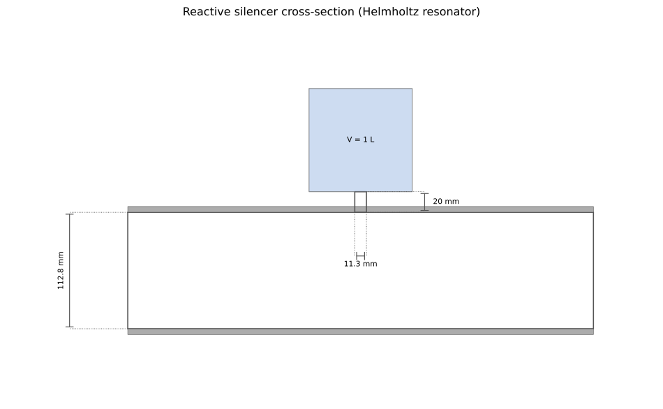
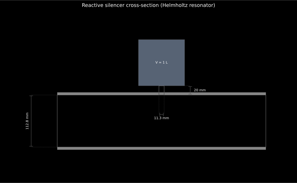
The whole 120 Hz notch hangs on a 1 L box and a 2 cm neck: the cavity is drawn as its equal-volume cube, and the tuning moves as , so small errors in these dimensions shift the spike off its target.
Show the code for this figure
import matplotlib.pyplot as pltimport numpy as npfrom phonometry import noise_control
f = np.linspace(20.0, 600.0, 4000)hr = noise_control.helmholtz_resonator(f, duct_area=0.01, neck_area=1e-4,                                       neck_length=0.02, cavity_volume=1e-3)
# One line: the side branch drawn to scale, cavity as its equal-volume cube.hr.plot_geometry()plt.show()
The quarter-wave tube needs no cavity at all: the 285 Hz spike of the figure above comes from a plain closed tube of the right length standing on the same duct.
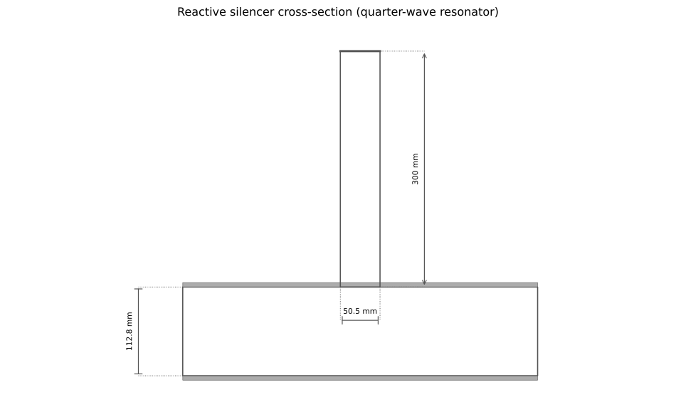
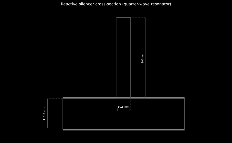
A quarter-wave stub is just a closed tube of the right length: 0.3 m of pipe puts the spike at , and the 20 cm² branch area only sets how strongly the stub loads the duct.
Show the code for this figure
import matplotlib.pyplot as pltimport numpy as npfrom phonometry import noise_control
f = np.linspace(20.0, 600.0, 4000)qw = noise_control.quarter_wave_resonator(f, duct_area=0.01, length=0.3, branch_area=2e-3)
# One line: the closed 0.3 m tube on its duct, to scale.qw.plot_geometry()plt.show()
Each returns a ReactiveSilencerResult with transmission_loss,
insertion_loss (when impedances are given), the compound transfer_matrix,
the plane_wave_limit of its widest cross section and .plot(). Layouts the four
constructors do not cover are chained element by element, either with the
bare duct_matrix, shunt_matrix, cascade, transmission_loss and
insertion_loss, or through SilencerChain, which makes the same calls and
keeps the geometry they were given.
That plane_wave_limit is the validity ceiling of everything on this page.
Above the first higher-order cut-on of the widest section several modes
propagate, each with its own axial wavenumber, and the computed peaks and
troughs do not survive; the result raises a PlaneWaveWarning when the analysis
grid runs past it. For the 0.04 m² chamber of the figures above the limit is
890.8 Hz, so the 2 kHz sweeps in the snippets are more than half outside the
model and the second and third peaks of the -family figure should be read as
design shape rather than prediction. The cut-on analysis itself is on
Duct-Borne Noise.
Three things about the hardware are outside the algebra and decide whether a
built device behaves like the curve. The shell of a chamber is a large
thin-walled radiator: if its own transmission loss is below the silencer’s, the
sound leaves through the shell and the device delivers the shell’s number, which
is the field version of the limiting insertion loss of section 3. The two
area discontinuities carry end corrections, exactly as a resonator neck
does, so the acoustic length exceeds the geometric one and the measured troughs
sit a little below the printed here; cut-and-try tuning has to be
verified rather than trusted. And the expansion regenerates flow noise at its
own outlet, which puts a floor under the delivered spectrum that the
transmission loss says nothing about; that quantity is
flow_noise_straight_duct on the
industrial noise-control page
and silencer_self_noise on the
duct-path page.
ReactiveSilencerResult also files itself: .report() renders a one-page PDF
in the layout of a silencer performance sheet, with the method-basis line
naming the plane-wave four-pole method (Munjal Eq. (3.27); Bies §8.8-8.9), an
optional metadata header (client, device, test environment, instrumentation,
climate, date), the per-band table of the transmission loss (and of the
insertion loss when the impedances were given) beside those same curves, the
boxed mean transmission loss over the analysis bands together with the peak
value and the device kind, and an optional verdict against a declared minimum
mean transmission loss. Rendering needs reportlab and, for the embedded
figure, matplotlib (pip install "phonometry[report,plot]"); pass
language="es" for a Spanish fiche.
import numpy as npfrom phonometry import ReportMetadata, noise_control
# A 0.5 m chamber of area ratio m = 8, at the octave-band centres.freqs = np.array([63.0, 125.0, 250.0, 500.0, 1000.0, 2000.0, 4000.0])res = noise_control.expansion_chamber(freqs, length=0.5, chamber_area=0.08, pipe_area=0.01)res.report(    "silencer_fiche.pdf",    metadata=ReportMetadata(        specimen="Simple expansion-chamber muffler (m = 8, design case)",        measurement_standard="Munjal Eq. (3.27) four-pole model",        laboratory="Phonometry Reference Laboratory",        requirement=6.0,            # minimum acceptable mean transmission loss    ),)                                   # mean and peak transmission loss (dB)
The example fiche is regenerated with make reports and kept rendered in the
repository; click the preview to open the PDF.
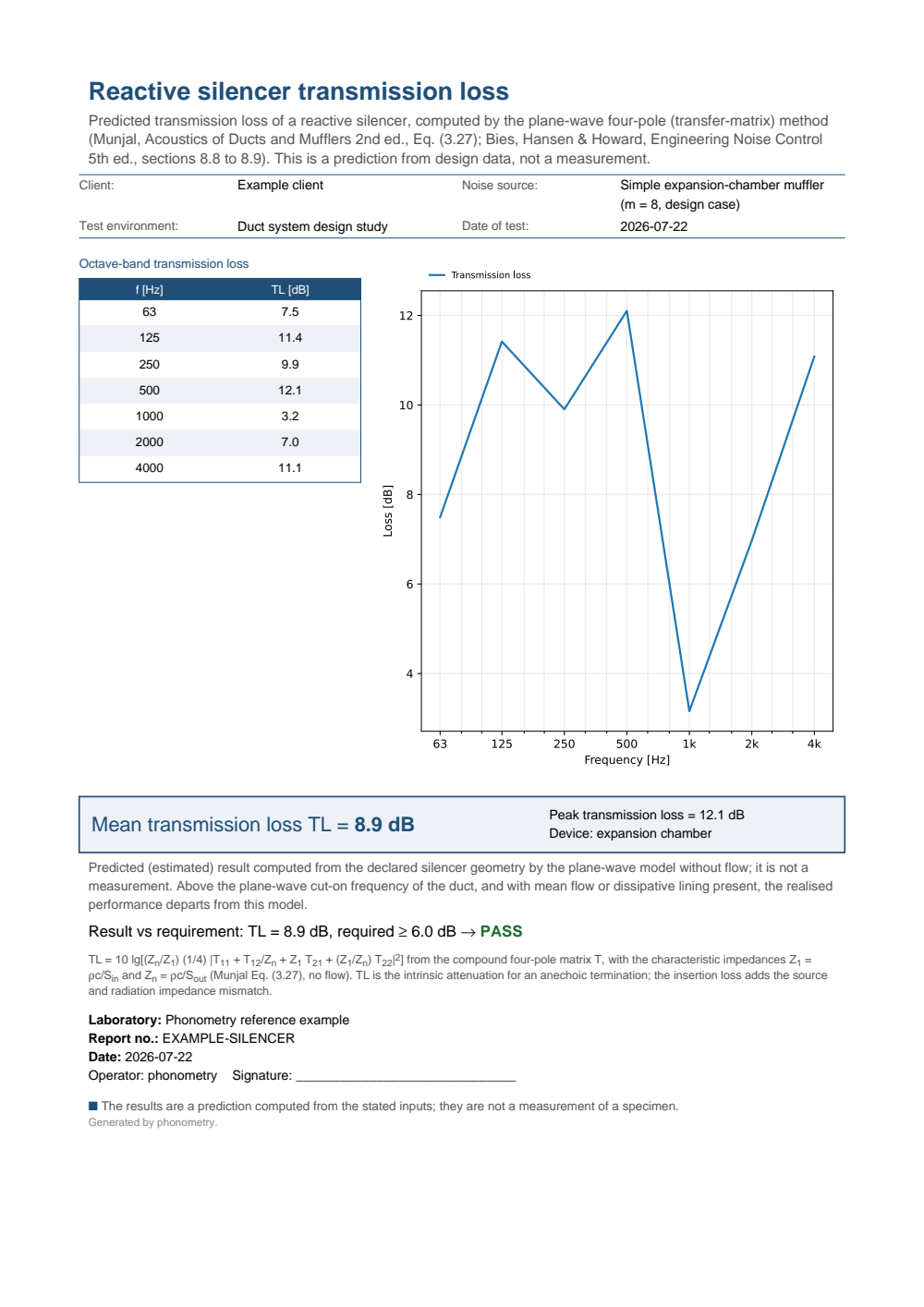
One-page reactive-silencer fiche: a metadata header with the client, the expansion-chamber muffler of area ratio m = 8 as the noise source, the duct-system design study and the test date, the octave-band transmission-loss table running 7.5, 11.4, 9.9, 12.1, 3.2, 7.0 and 11.1 dB from 63 Hz to 4 kHz beside the same curve plotted against frequency, the boxed mean transmission loss TL = 8.9 dB with the peak transmission loss of 12.1 dB and the device named as an expansion chamber, a PASS verdict against the required minimum of 6.0 dB, and the note that the result is a plane-wave prediction from the declared geometry and not a measurement.
Layouts of your own
Section titled “Layouts of your own”Nothing above covers a two-chamber muffler, or a chamber with a stub welded
onto its inlet pipe. Those are cascaded element by element, and SilencerChain
does it through the same duct_matrix, shunt_matrix and cascade calls
while keeping what each element was handed, so the layout can be drawn as well
as computed and the drawing cannot drift from the model.
What such a drawing may show follows from what the elements declare, and the
two kinds of element declare very different amounts. duct_matrix is handed a
length and an area, so a duct is drawn to scale, dimensioned, and its steps
with it. shunt_matrix is handed an impedance, which fixes no length, no area
and no volume: the Helmholtz resonator and the quarter-wave stub of the
previous section present the same kind of object to the chain, and a
perforate or an open end would present another. So a branch is marked at the
station where it joins the run, lettered with its name and with the one thing
its impedance does say about itself, the frequency at which it is least, where
the branch bites hardest, and nothing about it is dimensioned. The ends of the
run are left open for the same reason: a chain is a list of elements, not a
statement about the pipes it sits between. Put those pipes in the chain as duct
elements and they are drawn too. A chain that holds no duct of positive length
has no geometry and no scale to draw at, so it raises rather than drawing one.
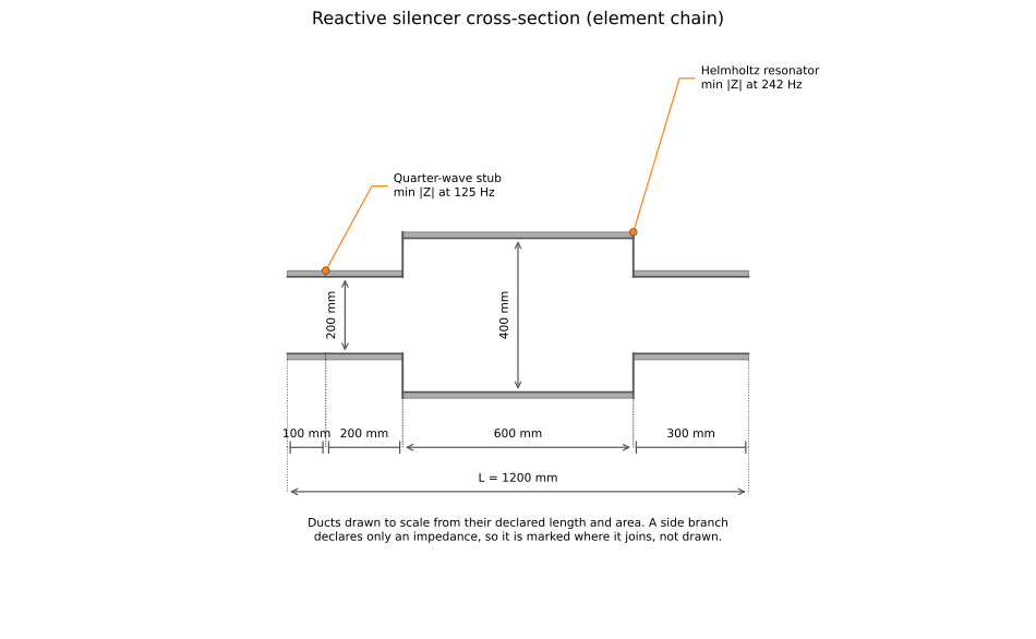
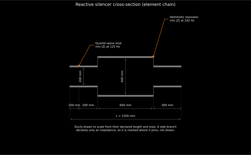
Every measurement on the page comes from what the chain was given: the four duct lengths and their sum are the numbers themselves, and the two bores are the areas it was handed, restated as the equivalent circular diameter . The two branches carry no dimension at all, because an impedance is not a shape.
Show the code for this figure
import matplotlib.pyplot as pltimport numpy as npfrom phonometry import noise_controlfrom phonometry.noise_control import helmholtz_impedance, quarter_wave_impedance
freqs = np.linspace(20.0, 500.0, 481)s_duct = np.pi * 0.100**2               # nominal 200 mm ducts_shell = np.pi * 0.200**2              # nominal 400 mm shell
# The elements in order, inlet to outlet; each call keeps what it was given.chain = (    noise_control.SilencerChain(freqs)    .duct(0.10, s_duct)    .shunt(quarter_wave_impedance(freqs, 343.0 / (4.0 * 125.0), np.pi * 0.050**2),           label="Quarter-wave stub")    .duct(0.20, s_duct)    .duct(0.60, s_shell)    .shunt(helmholtz_impedance(freqs, np.pi * 0.025**2, 0.05, 2e-3),           label="Helmholtz resonator")    .duct(0.30, s_duct))
# One line: the chain drawn exactly as it was declared.chain.plot_geometry()plt.show()
# The same elements evaluated: `.result()` gives the compound matrix, the# transmission loss, the plane-wave limit of the widest section, .plot() and# .report(), and `.transfer_matrix` alone is what `cascade` would have built.res = chain.result(inlet_area=s_duct, outlet_area=s_duct)res.plot()plt.show()
2. Reactive or dissipative?
Section titled “2. Reactive or dissipative?”Everything above works by reflection, and reflection has a shape: sharp, periodic, frequency-selective. The complementary family, dissipative silencers, replaces the impedance discontinuities with a duct section whose walls are lined with porous material (often protected by a perforated facing), so the grazing wave loses energy to viscous friction in the lining instead of being sent back to the source. The behaviours differ where it matters for selection:
- Frequency reach. A reactive chamber or resonator is strongest exactly where it is tuned and transparent elsewhere; a lined duct attenuates over a broad band that peaks where the lining depth is comparable with a quarter wavelength. At low frequency a practical lining is acoustically thin and does little, which is the regime where the reactive chamber wins; at high frequency the sound beams down the open airway and passes over the lining, so the attenuation of both families collapses and only splitter geometries (narrow airways, more lined perimeter per unit area) keep working.
- Spectrum type. A tonal source, an engine firing order or a blade-passing frequency, is a resonator’s natural prey; broadband fan or flow noise wants the dissipative band. Production exhaust silencers routinely combine the two, packing an expansion chamber with fibre so the reflective troughs of the chamber are filled by absorption.
- The medium. A porous lining in a hot, sooty or pulsating exhaust clogs and degrades, one reason vehicle exhausts are predominantly reactive; clean HVAC air is where dissipative attenuators and lined plenums are the default. In either case the airflow adds its own floor: a silencer regenerates flow noise at its own outlet, and past a certain pressure drop the silencer becomes the noise source.
Those are three frequency-dependent claims, so here they are on one axis, every curve computed from the shipped models rather than sketched.
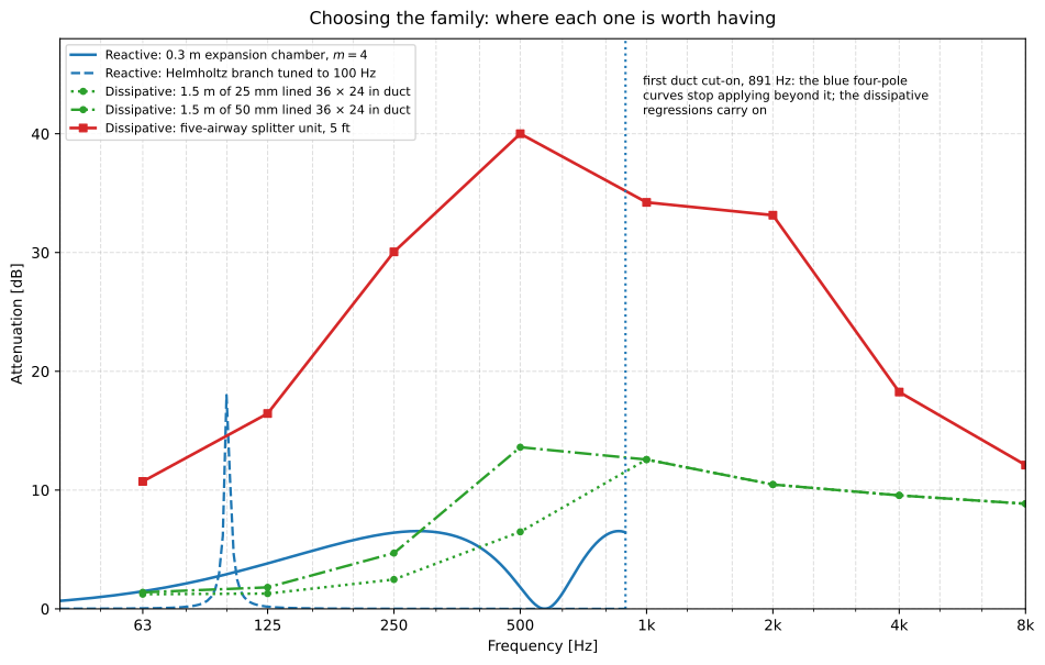
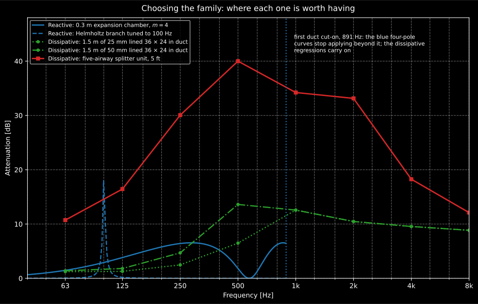
The selection rule, drawn. The resonator wins only where the tone is, and is transparent two semitones away. The chamber is worth a few decibels over a broad low band and nothing at all at its own half-wave troughs. A practical lining does almost nothing at 63 Hz (1.2 dB for 25 mm over 1.5 m) and doubling the lining thickness buys 7 dB at 500 Hz and nothing above 1 kHz, because there the sound already beams down the open airway. Only the splitter, which narrows the airway and multiplies the lined perimeter, keeps 30 dB through the middle. The blue curves stop at 891 Hz because that is where their model does.
Show the code for this figure
import matplotlib.pyplot as plt
# The reactive side, drawn only as far as its own validity ceiling.chamber = noise_control.expansion_chamber(f, 0.3, 0.04, 0.01)inside = f <= chamber.plane_wave_limit
fig, ax = plt.subplots()ax.semilogx(f[inside], chamber.transmission_loss[inside],            label="Expansion chamber, m = 4")ax.semilogx(f[inside], hr.transmission_loss[inside],            "--", label="Helmholtz branch")ax.set_xlabel("Frequency [Hz]"); ax.set_ylabel("Attenuation [dB]")ax.legend()plt.show()
The dissipative curves come from the installation models of the
HVAC methods, not from this
module: hvac.lined_rectangular_duct_attenuation(bands, 36 in, 24 in, 1.5 m, t, include_unlined=True) for the two linings, and
hvac.splitter_silencer_insertion_loss(bands, 24 in, 5 ft, [4 in] * 5, 8 in)
for the splitter unit.
phonometry models the reactive family in closed form on this page. The dissipative side enters at installation level, through the HVAC methods: the lined-elbow insertion loss read from tabulated ASHRAE data and the lined plenum attenuation from Wells’ closed form, neither of them a liner model. The porous physics that a first-principles liner calculation needs, the equivalent-fluid models fed by the airflow resistivity, is the same material theory as Porous and Multilayer Absorbers.
3. How a silencer is measured (ISO 7235)
Section titled “3. How a silencer is measured (ISO 7235)”Everything above is computed from geometry. The figure a supplier publishes is not: it is an insertion loss measured by substitution, and ISO 7235:2003 (published in Europe as EN ISO 7235:2009) is the method behind it. Reading the page’s fiche without knowing that is how a computed 8.9 dB and a catalogue “25 dB” end up in the same sentence.
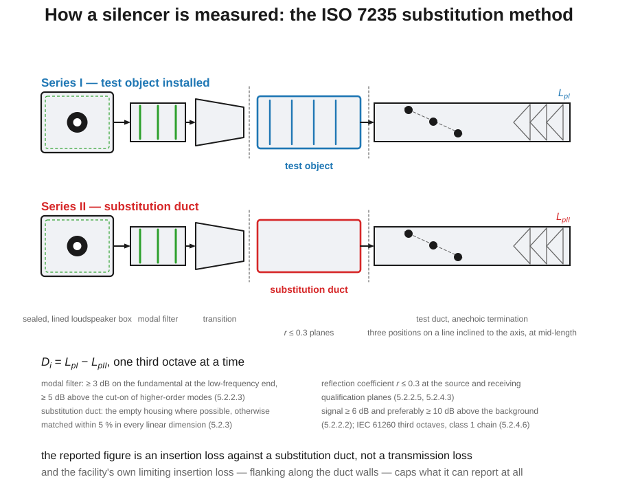
The rig has four parts and each of them carries a requirement. The source is a random-noise generator and amplifier driving loudspeakers in an acoustically sealed, absorbent-lined box, with pressure-equalisation openings for flow tests, powerful enough that every measurement point sits at least 6 dB and preferably 10 dB above the background (clause 5.2.2.2). A modal filter follows: a duct section with absorptive or reactive elements that attenuates the fundamental a little and higher-order modes a lot, at least 3 dB on the fundamental at the low-frequency end and at least 5 dB above the cut-on of higher-order modes, which also decouples the source from the test object (5.2.2.3). A rigid transition element joins them without radiating breakout noise (5.2.2.4). And the substitution duct is non-absorbent, ideally the empty housing of the test object itself, otherwise matched to its inlet and outlet within 5 % in every linear dimension (5.2.3).
The receiving side is one of three (5.2.4). A reverberation room to ISO 3741, qualified at least down to the 125 Hz third octave, is the preferred arrangement. A test duct with an anechoic termination is the fallback: at least half a wavelength of the lowest band long and at least four times the maximum cross dimension, with a reflection coefficient no greater than 0.3, and microphones plus fixtures obstructing under 5 % of the duct area. Essentially free-field conditions at the open end are allowed when the direct sound exceeds the strongest reflection by 10 dB, which holds when the nearest reflecting surface is more than twice as far away as the microphone.
The procedure is then two series with nothing else changed. is determined with the test object installed, with the substitution duct in its place, at identical points or paths and with an unchanged source spectrum, and the insertion loss is third octave by third octave (6.2.1). In a test duct the spatial average takes at least three equally spaced positions on a line inclined to the duct axis at about half its length, spanning at least a quarter wavelength of the lowest band, going to five when the spread between the three exceeds the Table 6 limits: 10 dB at 50 and 63 Hz, 8 dB at 80 and 100 Hz, 7 dB at 125 Hz and 6 dB above 160 Hz. The chain is class 1 with IEC 61260 third-octave filters (5.2.4.6) and is verified with a class 1 calibrator to dB before and after each series (6.1).
Two consequences travel with the number. First, what is reported is an insertion loss against a substitution duct, not a transmission loss, so it is not the quantity this page computes and the two must not be compared directly. Second, every facility has a limiting insertion loss, the ceiling set by flanking along its own duct walls, measured with the substitution duct acoustically blocked, and recorded as a function of frequency (7.4). A very large catalogue figure is a claim about the test arrangement as much as about the device, which is why the arrangement is reportable at all. For orientation on how repeatable any of this is, the standard’s own reproducibility standard deviations for insertion loss are 1.5 dB from 50 to 100 Hz, 1 dB from 125 to 500 Hz, 2 dB from 630 Hz to 1.25 kHz and 3 dB above (Table 7), with the expanded uncertainty twice those values.
Two neighbouring standards complete the picture: ISO 11691 is the survey- grade laboratory method without flow, and ISO 11820 measures a silencer in situ, where the substitution trick is usually impossible. The arithmetic of the first two, the subtraction itself and the tables that go with it, is on Measuring a Silencer.
Cross-check against the FDTD solver
Section titled “Cross-check against the FDTD solver”That cross-check is the clip embedded in section 1, and it is worth returning to it now with the algebra in hand. The four-pole expansion chamber is checked against the independent 2D FDTD wave solver, which shares no formula and no assumption with the transfer-matrix product beyond the wave equation itself: a plane-wave duct that widens into the same 0.30 m, chamber and narrows back transmits far less at the four-pole TL peak (, here 286 Hz) than at the transparent trough (, 572 Hz). The amplitude ratio measured downstream in the field is the transmission loss annotated on the clip, 6.5 dB at 286 Hz and 0.0 dB at 572 Hz, against the 6.55 dB the closed form gives for . Agreement that close rules out an algebra error on either side. The two must eventually part company above the duct’s first cut-on frequency, where higher-order modes propagate: the two-dimensional solver keeps working there and the plane-wave algebra does not.
What this guide covers
Section titled “What this guide covers”Covered
Reactive silencers by the four-pole transfer-matrix method (Bies §8.8-8.9, Munjal Eq. (3.27)): the closed-form
expansion_chamber(Eq. (8.111)),helmholtz_resonatorandquarter_wave_resonator(Eqs. (8.46), (8.44)),extended_tube_chamber, and theduct_matrix/shunt_matrix/cascade/transmission_loss/insertion_lossbuilding blocks for arbitrary element chains, gathered bySilencerChaininto a chain that keeps its geometry; the to-scale.plot_geometry()drawing on each of the four constructors’ results and on a chain, and the expansion chamber cross-checked against the independent FDTD solver; theplane_wave_limitthat bounds all of them; and, as prose rather than as code, the ISO 7235 substitution measurement that produces the insertion loss a supplier publishes, whose arithmetic is on its own page.Not covered
Only reactive elements are computed: dissipative (absorptive, duct-lining) silencers are discussed for selection but not modelled from the liner properties, and in the HVAC methods the lined-elbow figure is a table lookup (Bies Table 8.11) and the plenum attenuation is Wells’ closed form driven by a declared mean absorption; neither is a liner model. Mean-flow effects (convection, temperature gradients, flow-dependent impedance of perforates) are outside the no-flow element matrices used here. Nothing on this page is a measurement: the arithmetic of ISO 7235 has a page of its own, the shell breakout and the end corrections at the area jumps are not modelled, and the branch models are lossless unless a
resistanceis supplied.
References
Section titled “References”- Bies, D. A., Hansen, C. H., & Howard, C. Q. (2017). Engineering noise control (5th ed.). CRC Press. https://doi.org/10.1201/9781351228152The muffler four-pole method, the expansion-chamber TL and the resonator tuning formulas (§8.8-8.9) of this guide.
- International Organization for Standardization. (2003). Acoustics — Laboratory measurement procedures for ducted silencers and air-terminal units — Insertion loss, flow noise and total pressure loss (ISO 7235:2003 (EN ISO 7235:2009)). The substitution measurement of section 3: the source, modal filter, transition and substitution duct of Clause 5.2, the three receiving-side arrangements of 5.2.4, the two series of 6.2.1 with the Table 6 spread limits, and the limiting insertion loss of Clause 7.4 and Annex C.
- Munjal, M. L. (2014). Acoustics of ducts and mufflers (2nd ed.). Wiley. https://doi.org/10.1002/9781118443767The transfer-matrix formulation, the element matrices and the transmission loss from the compound matrix (Eq. (3.27)), and the reference treatment of dissipative and combined mufflers.
- Vér, I. L., & Beranek, L. L. (2006). Noise and vibration control engineering: Principles and applications (2nd ed.). Wiley. https://doi.org/10.1002/9780470172568The companion treatment of reactive and dissipative silencers.