Control Valve Noise (IEC 60534-8-3)

Standards: IEC 60534-8 IEC 61260Key references: Reethof & Ward 1986

A control valve is usually the loudest thing in a process plant, and it is loud for a reason worth stating plainly: throttling turns pressure into velocity, and the velocity is then thrown away in a free jet inside the pipe. A small and well characterised fraction of that jet’s power comes back as sound. The valve does not radiate it. The pipe does, which is why a prediction method that stops at the valve is not a prediction of anything anyone hears.

IEC 60534-8-3 is that chain, from an operating point to a level one metre from the pipe wall, and this page follows it.

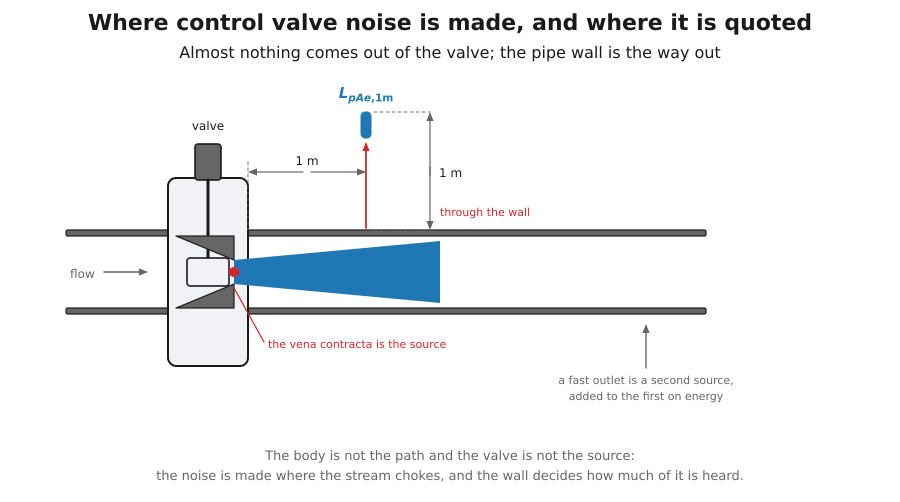
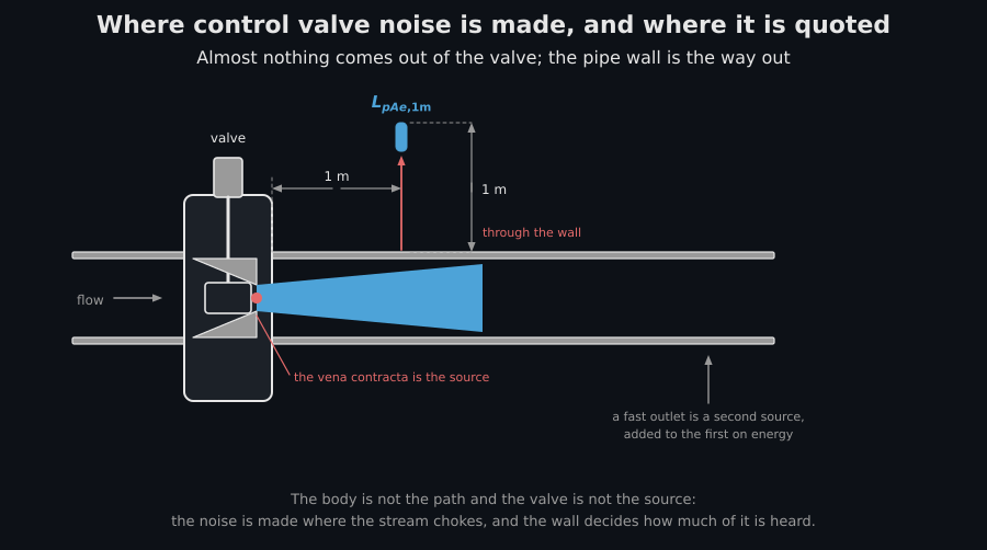
The whole of Clause 5 lives between those two points: what the jet makes, and what is left of it a metre outside the wall.

1. Five regimes, and why the method has a branch in it

Everything turns on the differential pressure ratio, Equation (1):

x = \frac{p _{1} - p _{2}}{p _{1}}

A valve barely throttling and a valve running a shock train are not the same noise source, and the standard does not pretend otherwise. Equations (3) to (7) cut $x$ into five intervals, and Table 3 gives each interval its own Mach number, its own acoustical efficiency and its own peak frequency.

Three panels. Left: the acoustical efficiency of one valve against the differential pressure ratio on a logarithmic axis, from one part in a million to two parts in a thousand, with the five regimes shaded and labelled with roman numerals and their four boundaries drawn as dotted lines. Middle: the sound pressure level in each one-third-octave band from 12.5 Hz to 20 kHz, once inside the pipe and once one metre outside it, about a hundred decibels lower, with the peak frequency marked. Right: the pipe transmission loss against frequency, rising from ninety decibels at the bottom of the range to a maximum near the internal coincidence frequency and falling again, with the external coincidence, internal coincidence and ring frequencies marked

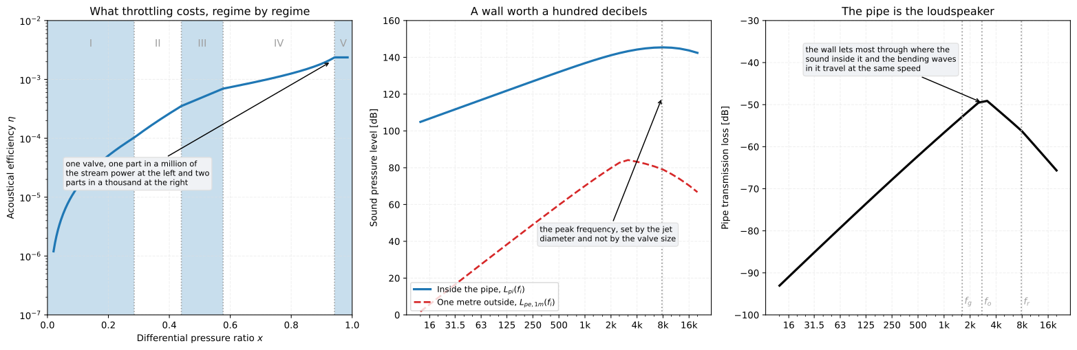
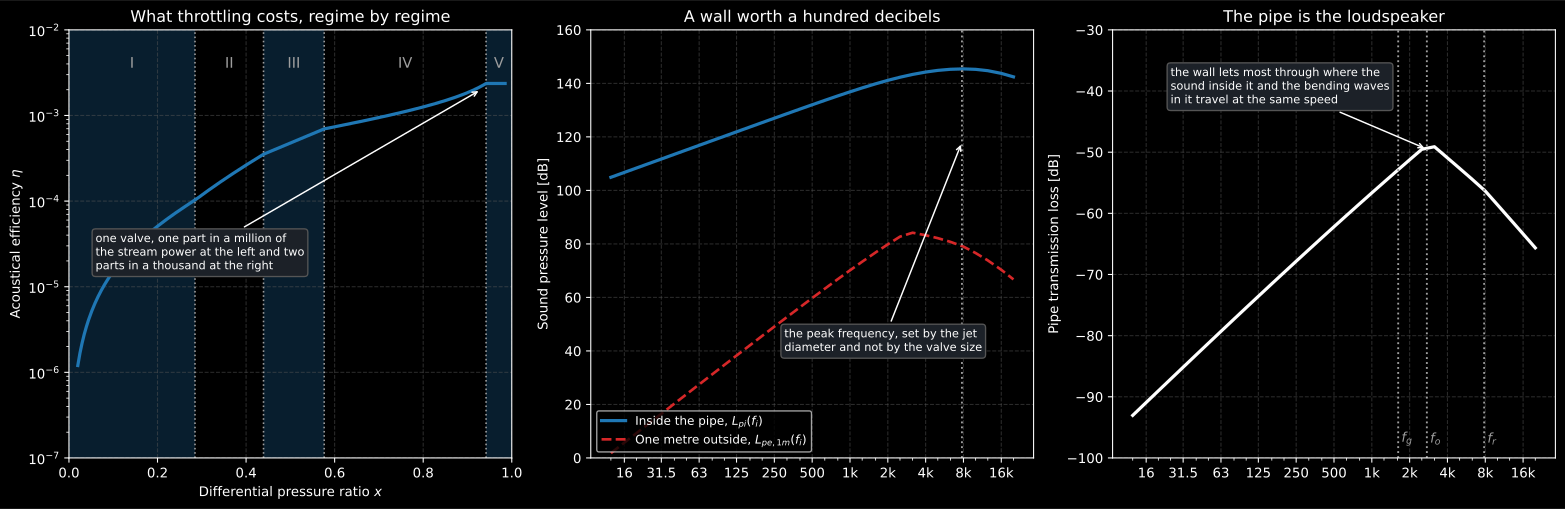
The same valve, from one part in a million of the stream power to two parts in a thousand, and the hundred decibels the pipe wall is worth.

The five are, in the order the clause prints them: I subsonic in the vena contracta, II and III choked with a jet that is still growing, and IV and V the shock-cell regimes, where the peak frequency stops following the jet velocity and starts following the spacing of the cells.

from phonometry import noise_control

bounds = noise_control.pressure_ratio_boundaries(1.22, 0.792 / 0.984)
print(round(bounds.critical, 3))              # 0.285  x_C
print(round(bounds.vena_contracta, 3))        # 0.439  x_vcc
print(round(bounds.break_point, 3))           # 0.576  x_B
print(round(bounds.constant_efficiency, 3))   # 0.942  x_CE

print(noise_control.flow_regime(0.28, bounds))   # 1
print(noise_control.flow_regime(0.52, bounds))   # 3
print(noise_control.flow_regime(0.95, bounds))   # 5

The second argument is the pressure recovery factor $F_{L}$ , or $F_{L P} / F_{p}$ when the valve has attached fittings, which is what the note to Table 3 asks for and what every example in Annex A uses.

The boundaries are printed twice and not identically. Clause 5.2 ends its list with “Regime V if $x_{C E} < x$ ” and Table 3 prints $x_{C E} \leq x$ for the same row, while its regime IV row ends $x \leq x_{C E}$ . Read as the table prints it, the single point $x = x_{C E}$ belongs to two regimes at once. The clause is the normative text and its list is consistent, so flow_regime follows the clause, and the errata register records the disagreement.

2. The jet, which is not the valve

The peak frequency of the noise is set by the size of one jet, not by the size of the valve. A cage with sixty small holes and a single-port plug of the same capacity make the same power and put it in very different places. Equations (8a) to (8c) are how the standard measures that:

d_{H} = \frac{4 A}{l _{w}}, d_{o} = \frac{4 N _{o} A}{π}, F_{d} = \frac{d _{H}}{d _{o}}

$d_{H}$ is the hydraulic diameter of one passage and $d_{o}$ the diameter of the single circular orifice that would pass the same total area, so $F_{d}$ is near one for a single large port and small for a cage.

from phonometry import noise_control

# The cage of Annex A: six openings, each 0,00137 m2 with a 0,181 m perimeter.
fd = noise_control.valve_style_modifier(0.00137, 0.181, 6)
print(round(fd, 3))                                        # 0.296

print(round(noise_control.jet_diameter_m(90.0, fd, 0.792 / 0.984), 4))
# 0.0116  m

Equation (9) then turns the flow coefficient into the jet diameter, $D_{j} = N_{14} F_{d} C F_{L P} / F_{P}$ , with $N_{14}$ from Table 1 by whichever coefficient the valve is rated in.

Annex A prints an orifice diameter ten times too small. Its Table A.1 gives $d_{o} = 0, 010$ m in all six columns where Equation (8c) with the annex’s own $N_{O} = 6$ and $A = 0, 00137$ m² gives $0, 102$ m. The row below settles it: the printed $F_{d} = 0, 30$ is $0, 030/0, 102$ , and it would be 3,0 with the printed $d_{o}$ . That one is in the errata register too, along with a piping geometry factor the annex prints rounded to 0,98 and computed with 0,984.

3. The whole of Clause 5, in one call

The rest of the chain is the acoustical efficiency of Table 3, the sound power of Equation (11), the internal level at the pipe wall of Equation (18), the spectrum of Equation (19), the pipe transmission loss of Equation (20a) and the level outside of Equations (24) and (25).

from phonometry import noise_control

result = noise_control.valve_aerodynamic_noise(
    noise_control.GasStream(
        mass_flow=2.22,                # kg/s
        inlet_pressure_pa=1.0e6,          # Pa, absolute
        outlet_pressure_pa=7.2e5,
        inlet_density=5.3,             # kg/m3
        inlet_temperature_k=450.0,       # K
        specific_heat_ratio=1.22,
        molecular_mass=19.8,           # kg/kmol
    ),
    noise_control.ValveTrim(
        flow_coefficient=90.0,         # C_v
        style_modifier=noise_control.valve_style_modifier(0.00137, 0.181, 6),
        pressure_recovery=0.792 / 0.984,
        outlet_diameter_m=0.1,           # m
        efficiency_correction=-3.8,    # A_eta, Table 4
        strouhal_number=0.2,           # St_p, Table 4
    ),
    noise_control.DownstreamPipe(
        internal_diameter_m=0.2031,      # m
        wall_thickness=0.008,          # m
        density=8000.0,                # kg/m3, steel
    ),
)

print(result.regime)                                # 1
print(round(result.sound_power, 1))                 # 22.3  W
print(round(result.internal_level, 1))              # 155.3 dB
print(round(result.peak_frequency))                 # 7778  Hz
print(round(result.external_level, 1))              # 91.7  dB

Every one of those is a printed value of Annex A’s example 1, including the last: the annex prints $L_{p A e, 1 m} = 92$ dB(A) for it. Five of the six columns end in a number Clause 5 alone reaches, and the library reproduces all five; the sixth is the one whose valve outlet is narrower than its pipe, so the annex adds the expander noise of Clause 7 to it, and Clause 5 by itself lands a decibel low. The result also carries the rest of the printed intermediates, so a calculation can be read against the standard row by row rather than trusted.

The last two arguments are the only ones a data sheet may not give. $A_{η}$ is the exponent of the acoustical efficiency and $S t_{p}$ the Strouhal number at the peak; Table 4 prints typical pairs for thirteen valve styles and says in its own NOTE 1 that a manufacturer states the real ones.

from phonometry import noise_control

print(noise_control.VALVE_ACOUSTIC_STYLES["globe ported cage"])
# (-3.8, 0.2)
print(noise_control.VALVE_ACOUSTIC_STYLES["segmented ball 90 deg"])
# (-3.6, 0.3)

$A_{η}$ is $- 4$ for a pure dipole, which is what a free jet expanding into a large volume is; the printed values run from $- 4, 8$ to $- 3, 0$ , so the whole table spans a factor of sixty in efficiency, which is 18 dB.

4. Where the sound actually comes out

The internal level is around 155 dB in the example above, and nobody standing beside the pipe hears anything like that. The pipe wall is what stands between them, and Equation (20a) is worth more than a hundred decibels at the bottom of the range.

It is not a flat hundred. Three frequencies shape it, and the middle one is where the wall gives most away:

f_{r} = \frac{c _{s}}{π D _{i}}, f_{o} = \frac{f _{r}}{4} (\frac{c _{2}}{c _{a}}), f_{g} = \frac{3}{π t _{S}} \frac{c _{a}^{2}}{c _{s}}

from phonometry import noise_control

pipe = noise_control.coincidence_frequencies(0.200, 0.008, 408.0)
print(round(pipe.ring))                    # 7958  Hz, f_r
print(round(pipe.internal_coincidence))    # 2366  Hz, f_o
print(round(pipe.external_coincidence))    # 1622  Hz, f_g

$f_{r}$ is the ring frequency, where the circumference is one wavelength in the steel. $f_{o}$ is the internal coincidence frequency, where the sound inside the pipe and the bending waves in its wall travel at the same speed, so they couple: that is the maximum in the right-hand panel of the figure, and it is where a valve’s noise gets out. $f_{g}$ is the external one, where the bending waves match the air outside.

import numpy as np
from phonometry import noise_control

bands = np.array([200.0, 1000.0, 2500.0])
loss = noise_control.pipe_transmission_loss(
    bands,
    internal_diameter_m=0.200,
    wall_thickness=0.008,
    valve_outlet_diameter_m=0.200,
    downstream_density=11.1,
    downstream_sound_speed=408.0,
    pipe_density=8000.0,
)
print(np.round(loss, 1))
# [-70.4 -56.9 -49.4]

All three are printed values of Annex A’s example 7. The loss is negative and Equation (24) adds it, which is the standard’s own sign and not a convention chosen here.

A thinner pipe is a louder pipe, and by a lot. The wall thickness enters Equation (20a) squared, so halving it is worth about 6 dB in every band, which is the cheapest and most often forgotten line in a valve noise budget.

5. When the outlet runs fast: the second source

Clause 5 has limits, and two of them bite. The pipe Mach number $M_{2}$ of Equation (17) is not really a limit but a clamp: NOTE 2 caps it at 0,3 before the velocity correction of Equation (16), however fast the pipe actually runs. The valve outlet Mach number $M_{o}$ of Equation (15) is a limit, and it is the one that matters, because past 0,3 the flow leaving the outlet stops being a detail and becomes a second noise source in its own right. NOTE 1 sends the calculation to Clause 7 for it.

from phonometry import noise_control

case = dict(
    stream=noise_control.GasStream(
        mass_flow=0.89, inlet_pressure_pa=1.0e6, outlet_pressure_pa=5.0e4,
        inlet_density=5.3, inlet_temperature_k=450.0, specific_heat_ratio=1.22,
        molecular_mass=19.8,
    ),
    valve=noise_control.ValveTrim(
        flow_coefficient=30.0,
        style_modifier=noise_control.valve_style_modifier(0.00137, 0.181, 6),
        pressure_recovery=0.792 / 0.984, outlet_diameter_m=0.1,
        efficiency_correction=-3.8, strouhal_number=0.2,
    ),
    pipe=noise_control.DownstreamPipe(
        internal_diameter_m=0.15, wall_thickness=0.008, density=8000.0
    ),
)
both = noise_control.valve_aerodynamic_noise(
    **case, expander=noise_control.Expander()
)

print(round(both.outlet_mach, 2))     # 0.89, far past the 0.3 of NOTE 1
print(round(both.pipe_mach, 2))       # 0.4, clamped to 0.3 for the correction
print(round(both.external_level))     # 94  dB(A), trim and outlet together

That is Annex A’s example 6, and 94 dB(A) is what the annex prints for it. Without the expander the same call gives 93 and warns that a source is missing: the level is the trim alone, which is not what a valve running at Mach 0,89 sounds like.

Clause 7 is a small chain of its own. The flow is accelerated through the narrower outlet, capped at Mach 0,8 in the pipe and at the speed of sound at the outlet, and what it makes is Equations (34) to (41):

U_{R} = \frac{U _{p} D _{i}^{2}}{β d _{i}^{2}}, W_{m R} = \frac{m ˙ U _{R}^{2}}{2} [(1 - \frac{d _{i}^{2}}{D _{i}^{2}})^{2} + 0, 2], η_{R} = 1 0^{A_{η}} M_{R}^{3}

from phonometry import noise_control

outlet = both.expander
print(round(outlet.inlet_velocity))            # 460  m/s
print(round(outlet.mach, 2))                   # 0.96
print(round(outlet.stream_power))              # 47854  W
print(round(outlet.sound_power, 1))            # 42.0   W
print(round(outlet.peak_frequency))            # 920    Hz
print(round(outlet.internal_level))            # 151    dB

Every one of those is printed in the sixth column of Table A.1. Note the company the outlet keeps: 42 W of sound against the 218 W the trim makes, but at 920 Hz instead of 7,9 kHz, which is why it moves the A-weighted answer at all.

The two sources add in energy, not in level. Equation (43) sums them inside the pipe, and Equation (24) then takes the sum through the wall once, because there is only one wall.

L_{p i S} (f_{i}) = 10 l g (1 0^{L_{p i} (f_{i}) /10} + 1 0^{L_{p i R} (f_{i}) /10})

Two other things about Clause 7 are worth knowing before using it. Its 7.1 limits the transition piece to 30 degrees of total included angle, because a steeper cone makes the flow unstable in ways the standard does not model. And the contraction coefficient $β$ of Equation (35) is a measurement, not a constant: NOTE 1 gives 0,93 for straight pattern globe valves, says some rotary valves may be as low as 0,7, and admits there are no data for the rest. Expander defaults to the 0,93 and to Table 4’s own expander row, which is $A_{η} = - 3, 0$ and not the valve’s figure.

6. Trims designed to be quiet

Everything above is Clause 5, which is a valve with ordinary trim. A valve bought to be quiet is not that, and Clause 6 says how it differs: not by a different method, but by what is fed into the same one.

There are three families and each substitutes something.

A drilled cage (6.2) makes many small jets instead of one large one, and Equation (26) replaces the pressure recovery factor of Equation (9) with a geometry, $[0, 9 - 0, 06 (l / d)]$ , where $l$ and $d$ are the length and diameter of one hole. A long hole recovers less than a short one, and NOTE 1 caps the ratio at 4 because the bracket would otherwise reach zero at 15.

from phonometry import noise_control

# 6.2's own example: 48 rectangular passages, 10 mm by 2 mm.
area = 0.010 * 0.002
perimeter = 2.0 * 0.010 + 2.0 * 0.002
print(round(4.0 * area / perimeter, 4))          # 0.0033  m, the hydraulic d
print(round(noise_control.multiple_passage_jet_diameter(
    90.0, 0.094, 0.020, 0.0033), 5))             # 0.00333 m

A multistage trim (6.3) drops most of its pressure before the stage that makes the noise, so the method is run on that stage: the stagnation pressure $p_{n}$ at its inlet stands in for $p_{1}$ , the density there for $ρ_{1}$ , and the flow coefficient of the last stage for the valve’s.

C_{n} = N_{16} A_{n}, p_{n} = (\frac{p _{1} C}{1 , 155 C _{n}})^{2} + p_{2}^{2}, ρ_{n} = ρ_{1} \frac{p _{n}}{p _{1}}

Which equation gives $p_{n}$ is a two-step reading and not a formula. NOTE 3 says that with $p_{1} / p_{2} \geq 2$ you assume $p_{n} / p_{2} < 2$ , take Equation (28a), and fall through to (28b) if the answer turns out to be $2 p_{2}$ or more; below a valve ratio of two, (28c) applies directly. The result says which branch it took, because a report should not have to guess.

from phonometry import noise_control

conditions = noise_control.multistage_trim_conditions(
    inlet_pressure_pa=7.0e6, outlet_pressure_pa=1.4e6, inlet_density=55.3,
    flow_coefficient=81.5,
    last_stage_coefficient=noise_control.last_stage_flow_coefficient(6.44e-3),
)
print(round(conditions.flow_coefficient))        # 315
print(round(conditions.stagnation_pressure_pa))     # 2102410  Pa
print(round(conditions.stagnation_density, 1))   # 16.6     kg/m3
print(conditions.equation)                       # 28a

Those three then go into the GasStream and the ValveTrim in place of the valve’s own inlet pressure, inlet density and flow coefficient. That is Annex A’s example 7, a 432-passage cage on a 70 bar vapour line, and it closes at the printed 89 dB(A) with a jet 2,2 mm across and a peak at 14,4 kHz.

A multipath, multistage trim (6.4) is both at once, and it is what example 7 actually is. It adds nothing new to the substitution: Equations (32) and (33) restate the regime I Mach number and peak frequency with the last stage’s recovery factor, which is what the substitution has already put there.

For 6.3 there is one thing more. Clause 5 has been run on the last stage alone, so Equation (31) puts the others back:

L_{p i} = L_{p i, n} + \frac{1}{( n - 1 ) ^{0, 125}} 10 l g \frac{p _{1}}{p _{n}}

from phonometry import noise_control

print(round(noise_control.stage_level_correction(150.0, 3, 7.0e6, 2.1e6), 1))
# 154.8  dB

The exponent is 0,125, so the number of stages barely enters: two stages and eight differ by a quarter of a term that is itself only a few decibels. What the correction really tracks is $p_{1} / p_{n}$ , the pressure the earlier stages took out.

What this guide covers

Covered
IEC 60534-8-3:2010, Clause 5, Clause 6 and the outlet-flow half of Clause 7, against all seven worked examples of Annex A. Clause 5 for a valve with standard trim: the pressure ratios of 5.1 and 5.2 with the five regimes they define, the valve style modifier and jet diameter of 5.3, the regime-dependent stream power, acoustical efficiency and peak frequency of Table 3, the internal level at the pipe wall of Equation (18), the third-octave spectrum of Equation (19), the pipe transmission loss of 5.5 with its ring and coincidence frequencies, and the external level of 5.6 in bands and as one A-weighted number. Clause 6 for a trim built to be quiet: the drilled cage of 6.2 with Equation (26), the multistage substitution of 6.3 with Equations (27) to (29) and its NOTE 3 branch, the stage correction of Equation (31), and the multipath multistage case of 6.4. And Clause 7 for the flow leaving the valve outlet once it passes Mach 0,3, with the transition piece, its stream power and efficiency, and Equation (43), which adds it to the trim inside the pipe.
Not covered yet
The experimentally determined efficiency factors of Clause 8, which are a laboratory procedure rather than a calculation; Clause 9, which combines a valve with two or more fixed-area stages installed downstream of it. The hydrodynamic case, where the fluid is a liquid and the sources are the turbulence of the jet and the cavitation that joins it once the corrected threshold is passed, is IEC 60534-8-4 and has a page of its own.

References

International Electrotechnical Commission. (2010). Industrial-process control valves — Part 8-3: Noise considerations — Control valve aerodynamic noise prediction method (IEC 60534-8-3:2010). The whole of this page: Clause 5 with its Tables 1, 3, 4, 5, 6 and 7, and the seven worked examples of Annex A.
International Electrotechnical Commission. (2014). Electroacoustics — Octave-band and fractional-octave-band filters — Part 1: Specifications (IEC 61260-1:2014). The 33 one-third-octave bands from 12,5 Hz to 20 kHz that Table 5 indexes and every spectrum on this page is carried on.
Reethof, G., & Ward, W. C. (1986). A theoretically based valve noise prediction method for compressible fluids. Journal of Vibration, Acoustics, Stress, and Reliability in Design, 108(3), 329-338. https://doi.org/10.1115/1.3269349Where the five regimes and the acoustical efficiency of each of them come from.

Created and maintained by José Manuel Requena Plens ORCID All projects