Loudspeaker Characterisation (IEC 60268-5)

A loudspeaker datasheet is a bundle of conventions, and IEC 60268-5 is the standard that fixes them: what “sensitivity” refers to, over which band a frequency range is read, how directivity is plotted and at what drive the distortion is measured. This guide covers the chain phonometry implements around a measured on-axis response: the sensitivity conventions where cross-datasheet comparisons usually go wrong, the baffled radiating piston that is the canonical physical model behind a cone’s radiation impedance and directivity, and the rated-characteristics report that renders the standard’s data sheet, with every panel drawn to the IEC 60263 scale conventions. A loudspeaker in a room with an open microphone is a closed loop rather than a datasheet, so the guide closes on Long’s gain-before-feedback criterion (Architectural Acoustics 2e, Ch. 18): the open-loop and feedback-loop gains, the 10 dB stability margin and the number-of-open-microphones correction. The distortion and frequency-response measurements that feed it live in Electroacoustics; the microphone counterpart has its own guide.

1. Sensitivity conventions (IEC 60268-5)

Distortion and response figures only compare across devices when the sensitivity conventions behind them match, and the loudspeaker convention is the one that trips people: a power-and-distance normalization with two independent traps in a single sentence of clause 20.3. (The microphone trap is the reference value, and it has its own section.)

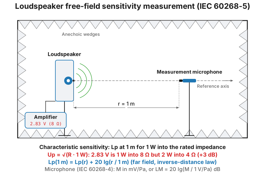
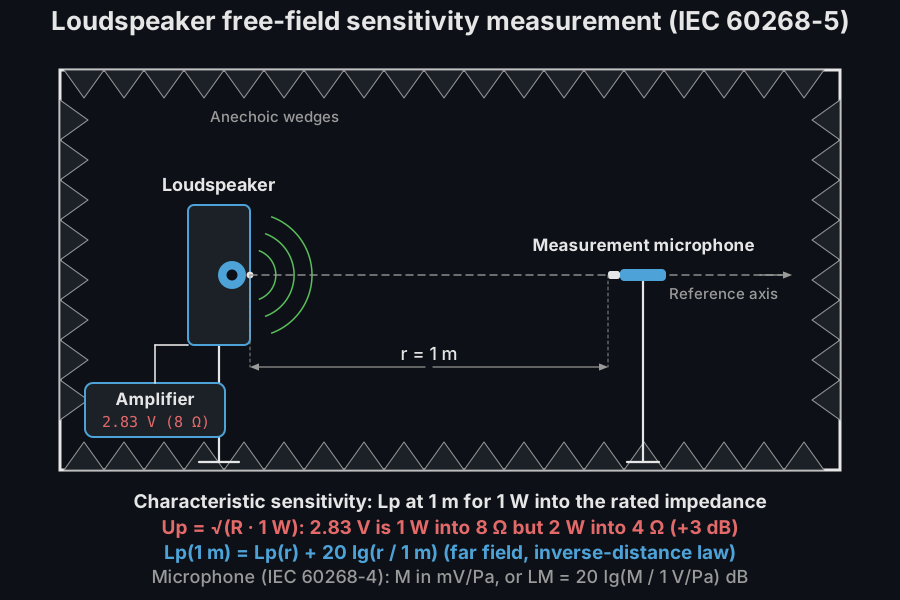
The trap the drawing exists to prevent is the 2.83 V one: that voltage is 1 W into 8 Ω and 2 W into 4 Ω, so the same figure flatters a 4 Ω loudspeaker by 3 dB.

The characteristic sensitivity is the sound pressure produced at 1 m on the reference axis, in the free field, referred to an input of 1 W into the rated impedance; expressed as a level re 20 µPa (clause 20.4) it is the familiar “dB @ 1 W/1 m”. Two normalizations hide in that sentence:

• The electrical one. The test voltage is $U_p=\sqrt{R\cdot 1\text{W}}$, numerically $\sqrt{R}$: 2.83 V into a rated 8 Ω. A datasheet quoting “dB @ 2.83 V/1 m” for a 4 Ω loudspeaker is feeding it 2 W, which flatters the figure by 3 dB against a true 1 W/1 m rating; check the rated impedance before comparing.
• The geometric one. 1 m is a reference distance, not necessarily the measurement distance. The standard has you measure in the far field (at 0.5 m or an integer number of metres, clause 7.1) and refer the result back with the inverse-distance law, $L_p(1\text{m})=L_p(r)+20{\log }_{10}(r/1\text{m})$. That scaling only holds where the level actually falls 6 dB per doubling of distance, hence the free field of the diagram; at 1 m from a large multi-way cabinet the near field may not have ended yet, and the quoted “1 m” figure is then a referred quantity, not what a microphone placed at 1 m would read.

1.1 How the on-axis curve is taken

Where “far field” starts. Section 1’s second bullet warns that a measurement can be too close without saying how close is too close. Three conditions have to hold together before the inverse-distance referral is legitimate: the distance must exceed a few times the largest dimension of the radiating surface, so the source subtends a small angle; it must exceed the wavelength at the lowest frequency of interest, so the reactive near field has decayed; and it must exceed the Rayleigh distance $\pi a^2/\lambda$ of the radiator, beyond which the on-axis pressure stops oscillating and settles into its $1/r$ decay. Work it for the 75 mm-radius piston of section 2 at 4 kHz: $\pi (0.075{)}^2/0.0858=0.21$ m, so 1 m is comfortably far. A 2 m tall column has not finished summing its drivers at 1 m at any frequency, and must be measured at 4 m or more and referred back — which is why clause 7.1.1 allows 0.5 m or an integral number of metres with a referral to the standard 1 m rather than insisting on 1 m, and why a datasheet “1 m” figure for a large cabinet is always a referred quantity.

Mounting, and the three reference geometries. The acoustic loading is part of the measured result, so clause 10.1 requires it to be described with the result and admits exactly three mountings for a drive unit: on a standard baffle, in a standard measuring enclosure (type A or B) or in a specified enclosure; in free air with no baffle at all; or flush with the reflecting plane in half-space free field. The three are not comparable — a unit measured in free air loses its whole low end to front-to-back cancellation, while the same unit flush in the plane gains the half-space 6 dB — and clause 11.1 notes that the radiating edge has to sit substantially flush with the front surface, by a chamfer or a thin rigid sub-baffle. A loudspeaker system is usually measured without any additional baffle (10.2). Clause 15 then defines the three things every distance and every angle on this page is measured from, and they are declarations by the manufacturer rather than measurements: the reference plane (15.1, tied to a physical feature of the unit or enclosure), the reference point on it (15.2), and the reference axis through that point (15.3), which is the zero of both the directional and the frequency-response measurements. Without them, “1 m” from the baffle, from the cone apex and from the cabinet back are three different sensitivities. Record where on the cabinet the reference point was placed. Clause 12 adds a preconditioning step before any of this: a simulated programme signal at the rated noise voltage for at least 1 h, then at least 1 h disconnected.

The excitation, which is not a sine. A characteristic sensitivity is measured with band-limited pink noise, not a swept tone (20.1.2): the chain is a pink-noise generator, a band-pass filter with slopes of at least 24 dB/octave limiting the signal to the band being measured, the loudspeaker, and the microphone at the stated distance; the drive is a stated voltage $U_p$, which for the characteristic sensitivity is numerically $\sqrt{R}$ (20.3.2). Where no filter of the right bandwidth exists, clause 20.1.2.4 gives the practical substitute: split the band into $n$ third-octave bands per IEC 61260, drive each at $U_p/\sqrt{n}$, and recombine as the r.m.s. of the band pressures. The instrument chain — generator, amplifier, loudspeaker, microphone amplifier — must be flat to ±0.5 dB over the range with negligible amplitude non-linearity, and all meters must be true r.m.s. (clause 8); the frequency range over which the total error stays inside ±2 dB has to be stated with the result (clause 9).

The gated measurement, for readers without an anechoic room. Clauses 5.5 and 7.3 admit simulated free field, which is how almost every response on the internet is actually taken: position the loudspeaker and the microphone so as to maximise the time before the first unwanted reflection reaches the microphone, and exclude everything from that arrival onwards by gating. The distance is then chosen to buy time rather than to be exactly 1 m, and referred back. Errors from wedge tips, the floor and the stands must stay under 0.5 dB (7.3), and the microphone distance and the maximum capture time the environment allows have to be stated with the result. The price is a hard low-frequency limit: a gate can only resolve a frequency whose period fits inside it, so a 5 ms reflection-free window — what a 1 m measurement at 1.2 m over a hard floor gives — is useless below roughly 200 Hz, and the low end has to come from a near-field or half-space measurement spliced in. That is also why a gated curve and an anechoic curve disagree below a few hundred hertz. The windowing machinery is the same as in Room impulse response.

2. Radiating piston: radiation impedance and directivity

The rigid circular piston in an infinite baffle is the canonical radiator behind a loudspeaker cone, the open end of a duct and the radiation efficiency of any finite vibrating surface (Beranek & Mellow §4.19, §13.7). Its mechanical radiation impedance is $Z_r=\rho cS(R_1+j{X}_1)$ with $S=\pi a^2$ and the dimensionless resistance and reactance functions (Eqs. (13.117), (13.118))

$$R_1(x)=1-\frac{2J_1(x)}{x},X_1(x)=\frac{2H_1(x)}{x},x=2ka,$$

where $J_1$ is the Bessel function and $H_1$ the Struve function of order one. At low frequency $R_1\to (ka{)}^2/2$ and the reactance is mass-like with the radiation mass $M_r=8\rho a^3/3$ (Eq. (4.151)); at high frequency $R_1\to 1$, $X_1\to 0$ and the piston radiates as if into an infinite tube. The far field follows the directivity $D(\theta )=2J_1(ka\sin \theta )/(ka\sin \theta )$, whose first null is at $ka\sin \theta =3.8317$.

import numpy as np
from phonometry import radiating_piston

res = radiating_piston(radius=0.075, frequencies=np.geomspace(20, 20000, 200),
                       angles=np.linspace(0.0, np.pi / 2, 91))
print(round(res.radiation_mass, 4))            # 0.0014 kg = 8 rho a^3 / 3
print(round(float(res.directivity_index[0]), 2))  # 3.01 dB half-space limit
res.plot()                                      # R1 and X1 vs ka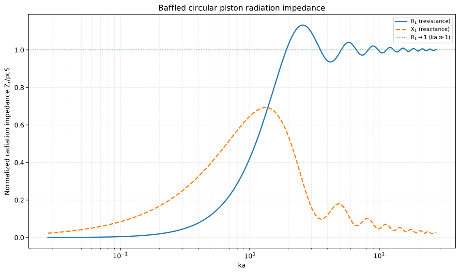

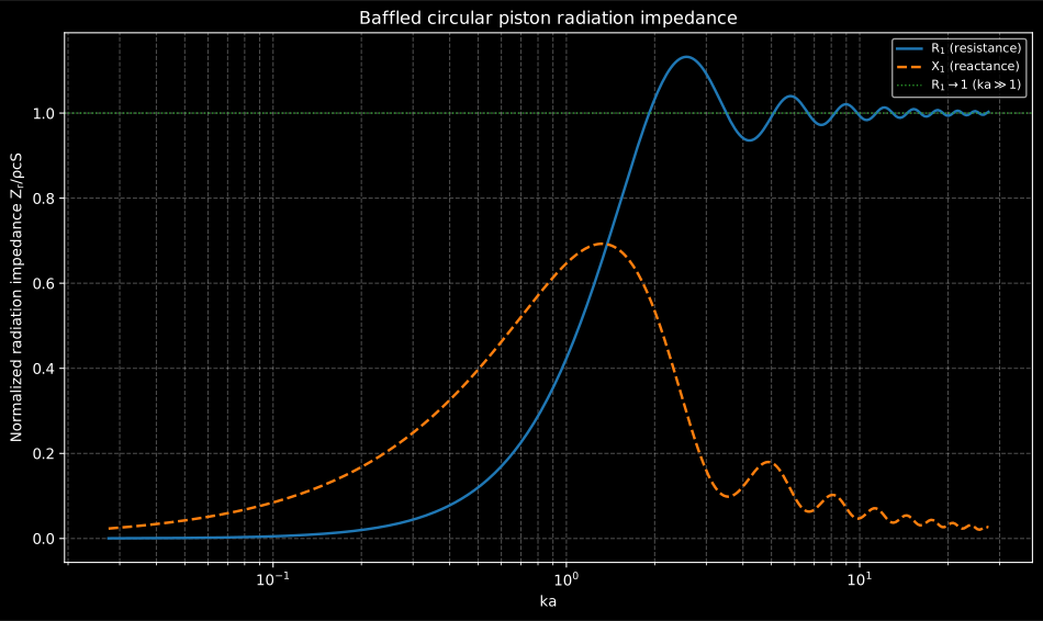
The .plot() of the 75 mm piston above is the classic Beranek & Mellow impedance figure: below $ka\approx 1$ the load is almost purely mass-like ($X_1$ dominates and $R_1\propto (ka{)}^2$, the regime where a loudspeaker’s output is stiffness- and mass-limited), and above it the resistance settles on $\rho cS$ with interference ripples while the reactance dies away.

The $ka$ axis reads as a frequency axis once the cone is fixed: $ka=1$ at $f=c/(2\pi a)$, which is 728 Hz for this 75 mm radius and 546 Hz for the 100 mm one of the geometry figure below. The directivity index printed by the snippet starts at 3.01 dB rather than 0 dB because a piston in an infinite baffle radiates into a half space, so even when it is omnidirectional within that half space it concentrates twice the power of a free-field point source, and $10{\log }_{10}2=3.01$ dB is the floor it rises from. The beamwidth follows the first null: the $-6$ dB half-angle narrows roughly as $\arcsin (2.2/ka)$, so a 100 mm cone is still hemispherical at 500 Hz and down to about 18° at 4 kHz — which is where a crossover to a smaller radiator has to happen.

Show the code for this figure

import matplotlib.pyplot as plt
import numpy as np
from phonometry import radiating_piston

res = radiating_piston(radius=0.075, frequencies=np.geomspace(20, 20000, 400))
res.plot()   # normalized R1 and X1 against ka
plt.show()

radiating_piston returns a RadiatingPistonResult with the normalized resistance/reactance, the mechanical radiation_resistance/radiation_reactance, the radiation_mass, the directivity_index, the far-field directivity pattern (when angles are given) and .plot(). The building blocks piston_resistance, piston_reactance, piston_directivity and plot_piston_geometry are also callable directly, the last of them without a result object at all. The piston is the companion radiator model of the reactive silencers.

Where the model stops

Every word of “rigid circular piston in an infinite baffle” is an assumption a real loudspeaker breaks, and each has a known failure. A cabinet is a finite baffle, so below the frequency whose wavelength exceeds the baffle width the radiation loads into $4\pi$ instead of $2\pi$ and the response falls by up to 6 dB — the baffle step — with edge diffraction adding a few decibels of ripple around it; none of that is in this model. A cone stops moving as one piece above its first breakup mode, typically a few times the $ka=1$ frequency for a paper cone, after which the real directivity is broader and more irregular than the Bessel pattern predicts. And a two-way system near its crossover is two sources, not one, so its polar response carries interference lobes a single piston cannot show, which is why the fiche’s polar panel is stated at a frequency. The model is exact where it is used here: as the radiation impedance of a small rigid surface, as the low-frequency directivity of a single driver on a large baffle, and as the reference case a measured directivity is read against.

The directivity pattern itself is a plottable result of its own: piston_directivity_pattern(ka) samples $D(\theta )$ at one or more $ka$ values and returns a PistonDirectivity (the polar angle grid, the linear directivity and its dB form directivity_db, and the ka values) whose .plot() draws the classic beam pattern. Several $ka$ are shown as one family on the same polar axes, so the narrowing of the main lobe and the emergence of the side lobes read at a glance:

from phonometry import piston_directivity_pattern

pattern = piston_directivity_pattern([3.0, 8.0, 16.0])
print(pattern.directivity_db.shape)  # (3, 361): one row per ka
pattern.plot()                       # polar beam pattern in dB (needs matplotlib)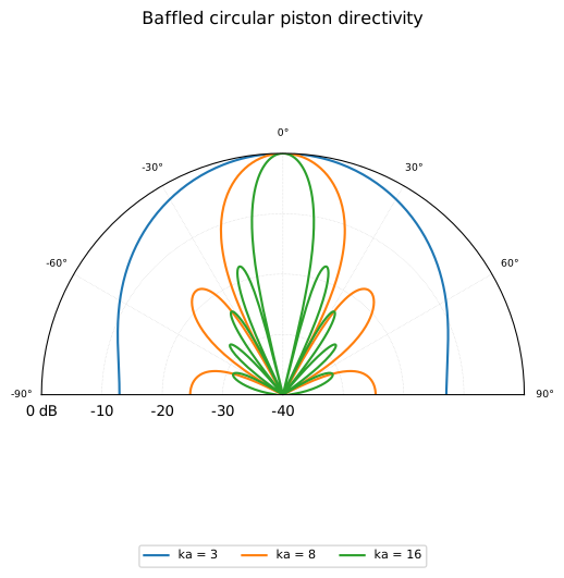

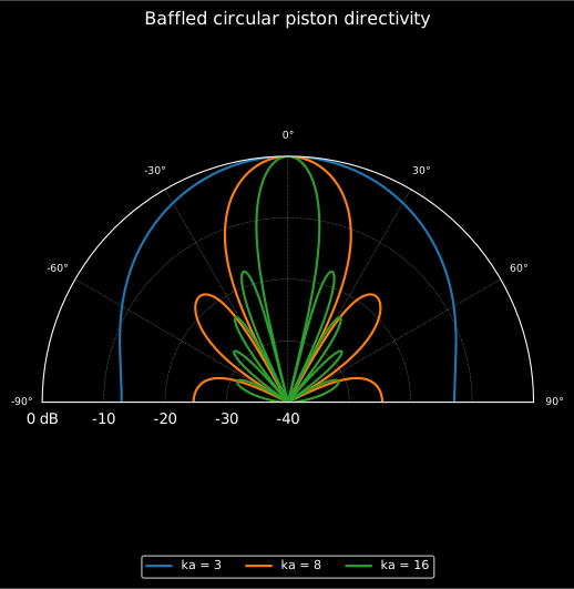
One piston at three frequencies, not three pistons: the first null tracks $ka\sin \theta =3.8317$, so a 75 mm-radius cone reaches $ka=16$ near 12 kHz and is by then radiating into a beam a few degrees wide.

Show the code for this figure

import matplotlib.pyplot as plt
from phonometry import piston_directivity_pattern

piston_directivity_pattern([3.0, 8.0, 16.0]).plot()
plt.show()

Behind both curves sits the same physical object, and .plot_geometry() on the piston result draws it: the plate in its rigid baffle to scale, with the far-field lobe of the highest computed frequency overlaid on the radiation side.

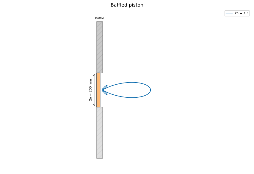
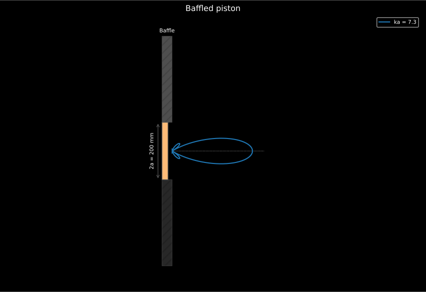
The piston the impedance and directivity curves describe, to scale: at 4 kHz this 10 cm radius plate has $ka\approx 7.3$, so the overlaid lobe is already several times narrower than the low-frequency hemisphere and the first side lobes have appeared.

Show the code for this figure

import matplotlib.pyplot as plt
import numpy as np
from phonometry import radiating_piston

res = radiating_piston(0.1, np.array([500.0, 2000.0, 4000.0]),
                       angles=np.linspace(-np.pi / 2, np.pi / 2, 181))

# One line: the piston in its baffle with the lobe of the highest frequency.
res.plot_geometry()
plt.show()

plot_piston_geometry(radius, angles=..., directivity=..., lobe_label=...) draws the same picture from a bare radius, with no RadiatingPistonResult at all, which is the form to reach for when sizing a cone or putting the baffle into a slide.

3. Loudspeaker characteristics report (IEC 60268-5)

The rated characteristics IEC 60268-5 defines around a measured on-axis response gather into a single loudspeaker characteristics result that renders the standard’s rated-characteristics data sheet. Two of the numbers are computed from the response rather than merely repeated:

• Characteristic sensitivity level (20.3/20.4). The on-axis level averaged over a stated band, referred to 1 W into the rated impedance $R$ at 1 m: $L_M=\overline{L}+20{\log }_{10}(d/d_0)+20{\log }_{10}(U_p/U)$ with $U_p=\sqrt{R\cdot 1\text{W}}=\sqrt{R}$. The default drive is that $\sqrt{R}$ (2.83 V into 8 Ω), so with a 1 m response the sensitivity level is the band mean.
• Effective frequency range (21.2). The band over which the response stays within 10 dB of the level averaged over the one-octave band in the region of maximum sensitivity; troughs narrower than 1/9 octave are neglected.

The rest of the fiche is a mixture of two kinds of number, and the standard draws the line clearly. The clause 20 and 21 quantities above are derived from the measurement. The clause 18 power ratings, the clause 19.1 rated frequency range and the clause 19.2 resonance frequency are declarations the manufacturer makes and the report prints; they are supplied through ratings=LoudspeakerRatings(frequency_range=..., noise_power=..., sinusoidal_power=..., resonance_frequency=...). The rated frequency range is not decoration: clause 16.1 applies the minimum-impedance criterion over that band, so omitting it makes minimum_impedance scan the whole measured curve and report a value the standard would not. The rated noise power and rated sinusoidal power come from the clause 17 endurance tests, which is why they are inputs here rather than outputs.

The 80 % line is an acceptance criterion, not decoration. Clause 16.1 says the rated impedance is a pure resistance the manufacturer declares, and constrains the declaration: the lowest modulus in the rated frequency range shall be not less than 80 % of it, and any dip below that value outside the range — d.c. included — shall be stated in the specification. That is the line drawn on the impedance panel, and minimum_impedance is exactly the quantity it is applied to. The consequence for whoever buys the loudspeaker is the minimum, not the rated, modulus: an “8 Ω” box dipping to 3.2 Ω is legal only if that dip lies outside the rated range, and an amplifier chosen on the nameplate figure may current-limit there. The same 80 % rule is why nominal 4 and 8 Ω ratings survive at all on a modulus that varies by an order of magnitude across the band.

Clause 16.2.2 fixes how the curve itself is taken: the loudspeaker under normal measuring conditions, driven at constant voltage or constant current — the former usually preferred — at a level small enough to keep it in a linear region, with the standard’s own warning that impedance is strongly influenced by drive level and that the data should be checked for consistency at several levels. The modulus is measured over at least 20 Hz to 20 kHz, and the voltage or current used is reported with the result.

import numpy as np
from phonometry import (
    LoudspeakerDirectivity, ReportMetadata, loudspeaker_characteristics,
    radiating_piston,
)

freqs = np.geomspace(30, 24000, 320)
spl = 87.0 + 1.2 * np.sin(2 * np.log2(freqs / 900.0))
spl -= 10 * np.log10(1 + (50.0 / freqs) ** 6)       # low-frequency roll-off
spl -= 10 * np.log10(1 + (freqs / 16000.0) ** 7)    # high-frequency roll-off

result = loudspeaker_characteristics(
    freqs, spl, rated_impedance=8.0, sensitivity_band=(200.0, 4000.0),
    impedance=(np.geomspace(20, 20000, 260),
               6.6 + 24 * np.exp(-(np.log2(np.geomspace(20, 20000, 260) / 52.0) ** 2) / 0.12)),
    distortion=(np.geomspace(50, 5000, 140),
                0.3 + 2.6 * np.exp(-(np.log2(np.geomspace(50, 5000, 140) / 70.0) ** 2) / 0.45)),
    directivity=LoudspeakerDirectivity(
        piston=radiating_piston(0.075, np.array([1000.0, 2000.0, 4000.0]),
                                angles=np.radians(np.linspace(0, 90, 46))),
        frequency=2000.0,
    ),
)
print(round(result.sensitivity_level_db, 1))                 # 87.1 dB, 1 W / 1 m
print(tuple(round(x) for x in result.effective_range))       # (37, 21361) Hz
print(round(result.minimum_impedance, 1))                    # 6.6 ohm

# The same response, but actually measured at 2 m with 1 V into 8 ohm.
referred = loudspeaker_characteristics(
    freqs, spl, rated_impedance=8.0, sensitivity_band=(200.0, 4000.0),
    distance=2.0, input_voltage=1.0,
)
print(round(referred.sensitivity_level_db, 1))               # 102.1 dB: +15.1

result.report("loudspeaker.pdf", metadata=ReportMetadata(measurement_standard="IEC 60268-5"))

distance is the distance the response was actually measured at and input_voltage the voltage it was driven with, and supplying them is how the two normalizations of section 1 are applied. The defaults are the 1 m, $\sqrt{R}$ case, so a 1 m response at 2.83 V into 8 Ω returns its own band mean unchanged. Measured at 2 m and 1 V instead, the same curve is referred up by 6.0 dB for the distance and 9.0 dB for the voltage — 15.1 dB in total, which is the size of error a reader would otherwise publish. One more input constraint, easy to miss: the band averages weight every sample equally, so a linearly spaced frequency axis puts most of its samples in the top octave and drags the sensitivity level towards the treble. That is why every example here builds its axis with np.geomspace.

loudspeaker_characteristics returns a LoudspeakerCharacteristics with the computed sensitivity_level_db, effective_range, reference_level_db, characteristic_sensitivity_pa and minimum_impedance, and a .report() that writes the fiche. The on-axis response is drawn with its tolerance band and the effective-range markers to the IEC 60263 proportion (one frequency decade equal to 25 dB), and the polar directivity on the IEC 60263 25 dB reference circle. The impedance modulus (with the 80 %-of-rated line), the total-harmonic-distortion curve and the directivity feed the secondary panels, reusing the radiating piston directivity of section 2 and a swept-sine THD result for the distortion curve.

The rated characteristics are also available interactively through .plot(), which draws one concept per figure with the same panel code the report composes, selected by quantity. Passing an axes draws on it:

result.plot()                        # on-axis response (default)
result.plot(quantity="impedance")    # |Z| modulus with the rated / 80 % lines
result.plot(quantity="thd")          # total harmonic distortion vs frequency
result.plot(quantity="directivity")  # polar response on the 25 dB circle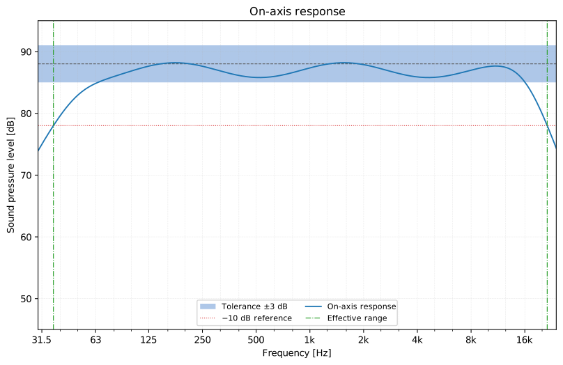

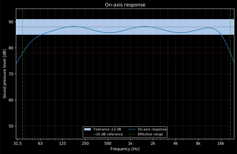
The ordinate is compressed to the IEC 60263 proportion of one frequency decade per 25 dB, which is what makes two datasheets comparable by eye. The shaded band is the $\pm$ tolerance the caller declares (tolerance_db, 3 dB here) and the markers are the clause 21.2 effective-range edges, read against the $-10$ dB line referred to the octave of maximum sensitivity — not to the mean of the whole curve.

Show the code for this figure

import matplotlib.pyplot as plt
import numpy as np
from phonometry import loudspeaker_characteristics

freqs = np.geomspace(30, 24000, 320)
spl = 87.0 + 1.2 * np.sin(2 * np.log2(freqs / 900.0))
spl -= 10 * np.log10(1 + (50.0 / freqs) ** 6)       # low-frequency roll-off
spl -= 10 * np.log10(1 + (freqs / 16000.0) ** 7)    # high-frequency roll-off

result = loudspeaker_characteristics(freqs, spl, rated_impedance=8.0,
                                     sensitivity_band=(200.0, 4000.0))
result.plot()   # quantity="response" (the default)
plt.show()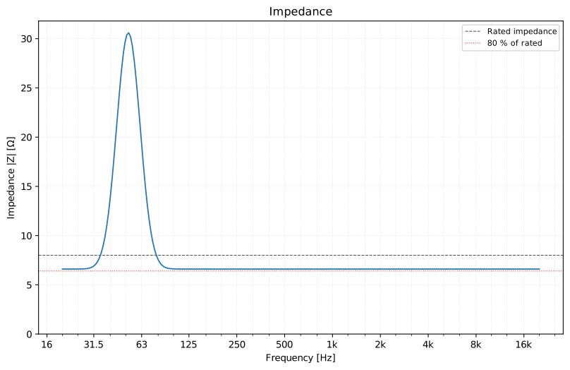

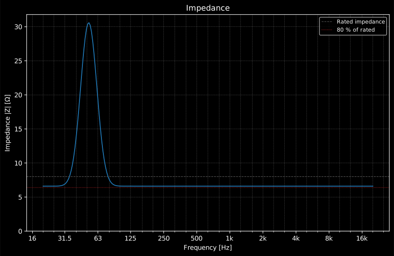
The peak at 52 Hz in this example is the driver’s fundamental resonance, where the moving mass and the suspension compliance exchange energy and the motor’s back-EMF is largest — the rating is not allowed to be read there. The 80 % line is the clause 16.1 acceptance limit, and the minimum modulus, not the rated one, is the load the amplifier actually sees.

Show the code for this figure

import matplotlib.pyplot as plt
import numpy as np
from phonometry import loudspeaker_characteristics

freqs = np.geomspace(30, 24000, 320)
spl = 87.0 - 10 * np.log10(1 + (50.0 / freqs) ** 6)
fz = np.geomspace(20, 20000, 260)

result = loudspeaker_characteristics(
    freqs, spl, rated_impedance=8.0, sensitivity_band=(200.0, 4000.0),
    impedance=(fz, 6.6 + 24 * np.exp(-(np.log2(fz / 52.0) ** 2) / 0.12)),
)
result.plot(quantity="impedance")
plt.show()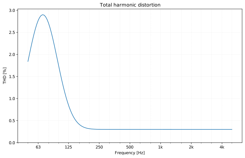

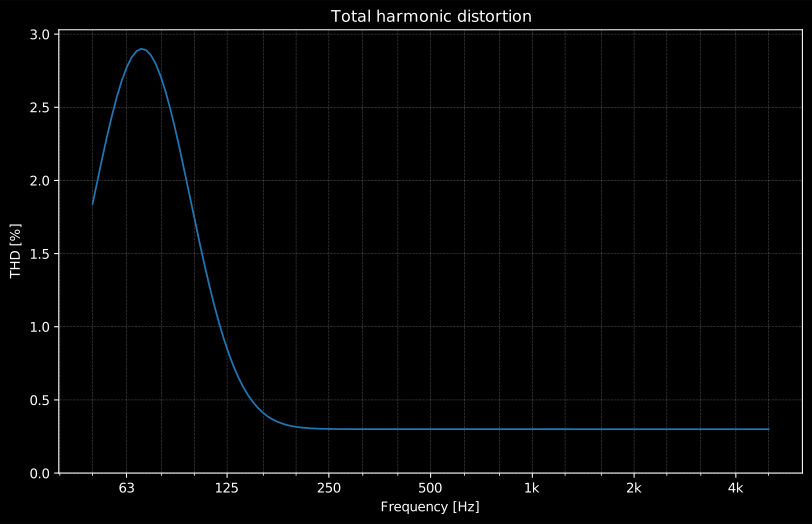
Read against the response above it: a distortion peak coinciding with a response peak is a resonance being driven hard, and a rise towards low frequency is the cone running out of excursion. Distortion is quoted at a stated drive, so a THD curve without its input voltage and the sound pressure level it produced at 1 m is uninterpretable (clause 24.1.2.7).

Show the code for this figure

import matplotlib.pyplot as plt
import numpy as np
from phonometry import loudspeaker_characteristics

freqs = np.geomspace(30, 24000, 320)
spl = 87.0 - 10 * np.log10(1 + (50.0 / freqs) ** 6)
thd_f = np.geomspace(50, 5000, 140)

result = loudspeaker_characteristics(
    freqs, spl, rated_impedance=8.0, sensitivity_band=(200.0, 4000.0),
    distortion=(thd_f, 0.3 + 2.6 * np.exp(-(np.log2(thd_f / 70.0) ** 2) / 0.45)),
)
result.plot(quantity="thd")
plt.show()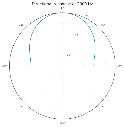

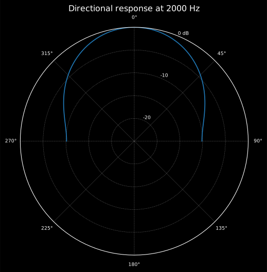
Drawn on the IEC 60263 clause 3 reference circle: the full radius is 25 dB and each ring is 5 dB, so the $-6$ dB half-angle — the coverage number a system designer works with — can be read straight off. The polar zero is the reference-axis level, which is why the drive has to be retrimmed per band while the cut is taken.

The panel is one cut, and clause 23.1.2 says how a cut is taken:

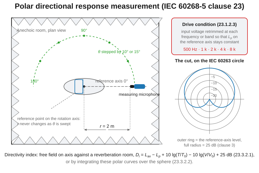
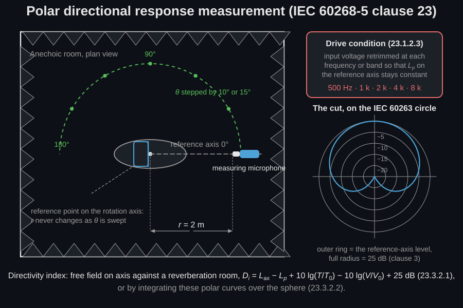
The loudspeaker turns and the microphone does not: the reference point sits on the rotation axis so the measuring distance never changes as $\theta$ is swept (23.1.2.2). The rule that makes the result a pattern rather than a family of responses is 23.1.2.3 — the input voltage is retrimmed at each frequency or band so that the sound pressure at a specified point on the reference axis stays constant — and the preferred display is a family of polar curves at stated bands, at least 500 Hz, 1, 2, 4 and 8 kHz, with the reference-axis level as the zero of the diagram. The step-by-step variant of clause 13.1.2 of the microphone standard uses 10° or 15°; here 23.1.2.4 recommends a device giving continuous angular variation, with the frequency-response variant at 15° intervals.

The directivity index the fiche prints has two admissible routes (23.3.2). Either measure the on-axis level at 1 m in a free field and the level of the same loudspeaker in a reverberation room, and correct: $D_i=L_{ax}-L_p+10\lg (T/T_0)-10\lg (V/V_0)+25$ dB, with $T_0=1$ s and $V_0=1{\mathrm{m}}^3$; or integrate the squared pressures of these polar curves over the sphere. LoudspeakerDirectivity takes either an already computed index_db, or the polar data the second route needs.

Show the code for this figure

import matplotlib.pyplot as plt
import numpy as np
from phonometry import (
    LoudspeakerDirectivity, loudspeaker_characteristics, radiating_piston,
)

freqs = np.geomspace(30, 24000, 320)
spl = 87.0 - 10 * np.log10(1 + (50.0 / freqs) ** 6)

result = loudspeaker_characteristics(
    freqs, spl, rated_impedance=8.0, sensitivity_band=(200.0, 4000.0),
    directivity=LoudspeakerDirectivity(
        piston=radiating_piston(0.075, np.array([1000.0, 2000.0, 4000.0]),
                                angles=np.radians(np.linspace(0, 90, 46))),
        frequency=2000.0,
    ),
)
result.plot(quantity="directivity")
plt.show()

The example fiche is regenerated with make reports and kept rendered in the repository; click the preview to open the PDF.

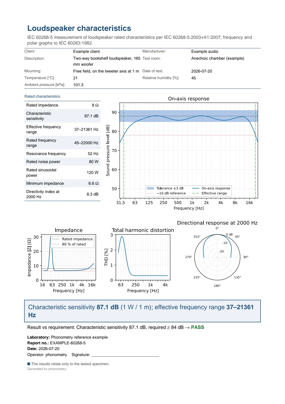
One-page IEC 60268-5 loudspeaker rated-characteristics fiche: a header with the manufacturer and model, the rated-characteristics table (rated impedance, characteristic sensitivity, effective and rated frequency ranges, resonance frequency, rated powers, minimum impedance and directivity index) beside the on-axis frequency response with its tolerance band and effective-range markers, and the impedance, total-harmonic-distortion and polar-directivity panels, all drawn to the IEC 60263 scale conventions.

Download the report (PDF)

Loudspeaker characteristics fiche (LoudspeakerCharacteristics.report), the IEC 60268-5 rated-characteristics table beside the on-axis response, impedance, THD and polar panels drawn to the IEC 60263 25 dB-per-decade and 25 dB reference-circle conventions.

4. Gain before feedback of a reinforcement system

All of that describes the device on a stand. Put it in a room with an open microphone and the governing number is no longer on the datasheet: the system is a closed loop: the loudspeaker feeds the audience, and it also feeds the microphone that drives it. Long (Architectural Acoustics 2e, Ch. 18, Eqs. (18.13) to (18.24)) writes that loop with two decibel gains. The open-loop system gain is what the system buys the talker,

$$Z_S=L_{H\text{-}L}-L_{T\text{-}M},$$

the level the loudspeaker produces at an average listener minus the level the talker produces at the microphone; $Z_S=-6$ dB, typical of an auditorium or a church, means a comfortable conversational level at twice the talker-to-microphone distance. The feedback-loop gain is the part of the output that comes back,

$$G_S=L_{H\text{-}M}-L_{H\text{-}L}+D_M(\theta ),$$

with $D_M(\theta )$ the directivity index of the microphone toward the loudspeaker relative to the talker: zero for an omnidirectional microphone, about $-2$ to $-3$ dB for a cardioid pointed at the talker. Summing the infinite series of round trips, the system oscillates when the loop gain reaches unity, that is $Z_S+G_S=0$ (Eq. (18.16)).

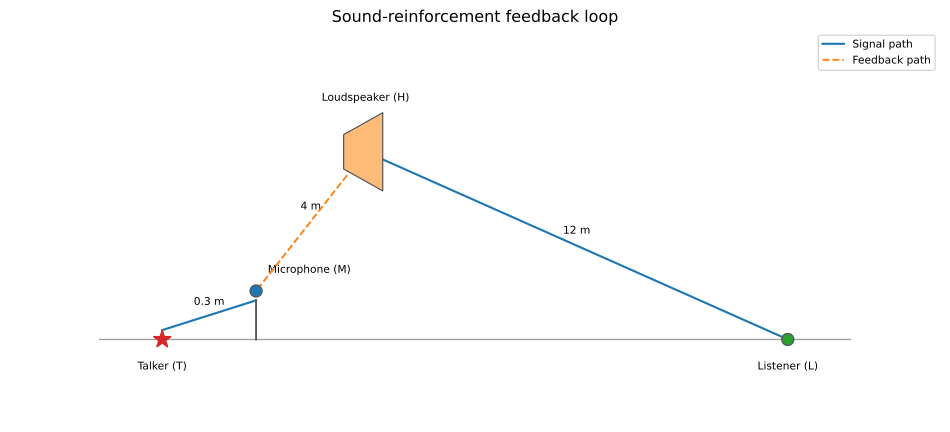
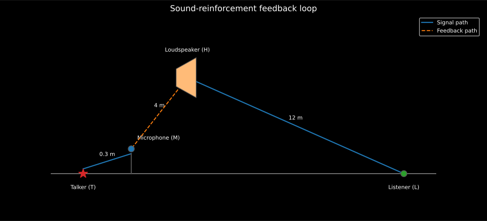
The four points of the loop. Only the sound field the loudspeaker produces at two of them, and the type and orientation of the microphone, enter the criterion: the loudspeaker’s own type, number and power do not appear anywhere in it.

A working system needs margin below that threshold. Long takes 10 dB for an equalized system (other authors quote 12 dB unequalized and 6 dB carefully equalized): 6 dB of it covers a sustained tone adding in phase with a reflection off a hard surface, and the remaining 4 dB is safety. With several microphones open at once the returned signals add at the mixer, which the number-of-open-microphones correction $\Delta L_{\text{nom}}=10{\log }_{10}{N}_m$ accounts for (Eq. (18.23)). The criterion is then

$$Z_S+L_{H\text{-}M}+\Delta L_{\text{nom}}\le L_{H\text{-}L}-D_M(\theta )-10.$$

from phonometry import electroacoustics as ea

# An auditorium at Zs = -6 dB, omnidirectional microphone, one mic open.
res = ea.feedback_stability(-6.0, 76.0, 80.0)
print(res.is_stable, round(res.headroom, 1))          # True 0.0 dB
print(round(res.maximum_level_at_microphone, 1))      # 76.0 dB = L(H-L) - 4

# A cardioid buys back exactly its relative directivity index.
card = ea.feedback_stability(-6.0, 78.0, 80.0, microphone_directivity=-2.0)
print(round(card.maximum_level_at_microphone, 1))     # 78.0 dB = L(H-L) - 2

# Four open microphones cost 10 lg 4 = 6 dB of that headroom.
print(round(ea.open_microphone_correction(4), 1))     # 6.0 dB

res.plot()      # the gain structure against the oscillation and margin lines

The bar stack below is the bookkeeping, and it is a level. What it cannot show is why the threshold sits at unity rather than anywhere else, because that is a statement about a sequence: the talker’s burst reaches the microphone, goes out of the loudspeaker, comes back to the microphone reduced by the loop gain, and does it again. Successive round trips either shrink, in which case the sum of all of them is finite, or they do not, in which case there is no sum. Watching the copies is the whole argument.

A burst circulates the loudspeaker-to-microphone path while each returning copy is drawn as a stem and the running total of all copies so far is plotted. With Long's 10 dB margin each copy is 0.316 of the last and the total settles 3.30 dB above the direct sound; four open microphones add 6 dB and the same loop takes far longer to settle, 8.69 dB up; four more decibels of system gain put the loop gain at unity, the copies stop shrinking and the total climbs without limit.

Download the animation (WebM)

A burst circulates the loudspeaker-to-microphone path while each returning copy is drawn as a stem and the running total of all copies so far is plotted. With Long's 10 dB margin each copy is 0.316 of the last and the total settles 3.30 dB above the direct sound; four open microphones add 6 dB and the same loop takes far longer to settle, 8.69 dB up; four more decibels of system gain put the loop gain at unity, the copies stop shrinking and the total climbs without limit.

Download the animation (WebM)

Three runs of the same auditorium, all from feedback_stability with $L_{H\text{-}M}=76$ dB and $L_{H\text{-}L}=80$ dB. The loop gains are $-10.0$, $-3.98$ and $+0.02$ dB, so each round trip multiplies the last by 0.316, 0.632 and 1.002; the first two sums converge to $1/(1-g)$ and the third does not converge at all. That is why gain before feedback is not a level limit: 6 dB more amplifier moves every copy up together and changes nothing about whether the series converges, while 6 dB more loop gain is the difference between a system and a howl.

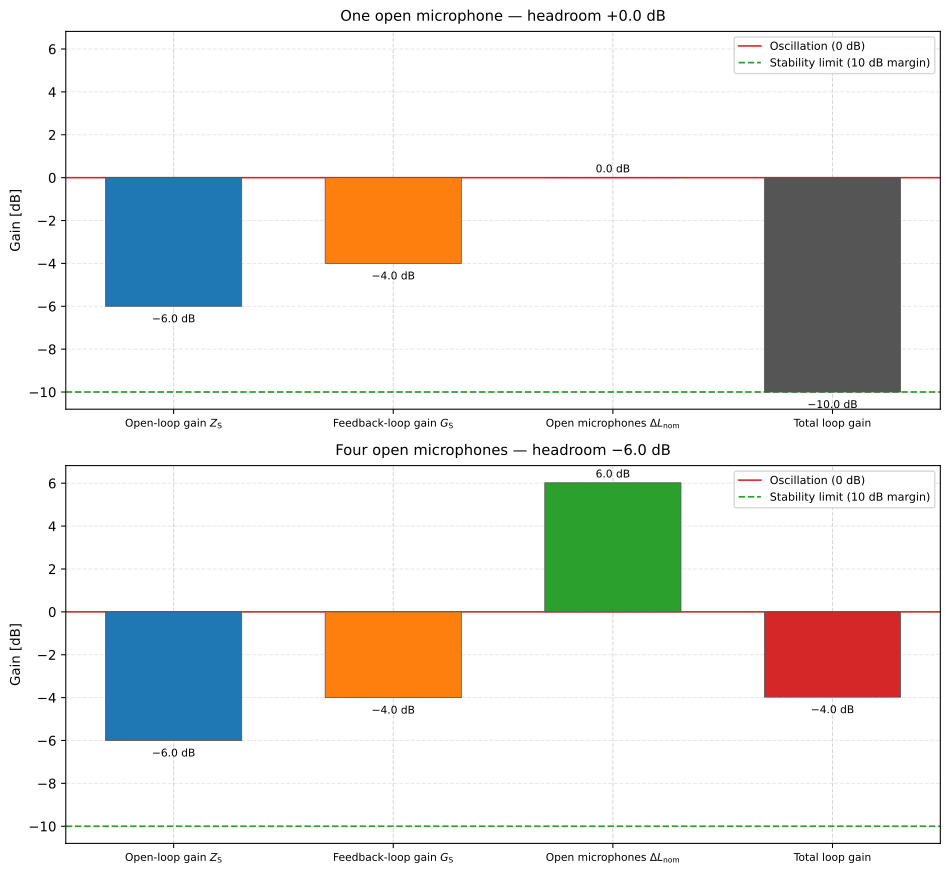
The loudspeaker’s type, its number and its power appear nowhere in the stack, which is why more amplifier never buys gain before feedback. Opening four microphones instead of one adds $10\lg 4=6$ dB and eats the whole margin: the same room, the same loudspeaker, the same talker, and a system that now rings. Long splits the 10 dB itself into 6 dB for a sustained tone adding in phase with a hard-surface reflection and 4 dB of safety.

Show the code for this figure

import matplotlib.pyplot as plt

# `ea` as imported above.
fig, axes = plt.subplots(2, 1, sharey=True)
ea.feedback_stability(-6.0, 76.0, 80.0).plot(ax=axes[0])
ea.feedback_stability(-6.0, 76.0, 80.0, open_microphones=4).plot(ax=axes[1])
plt.show()

Obtaining the four inputs

The criterion consumes three levels and a directivity index, and all four are measurements rather than assumptions. Take them in this order.

1. Set the system once and do not touch it. $L_{H\text{-}M}$ and $L_{H\text{-}L}$ are a pair read at one unchanged gain setting, so only their difference matters and a relative reading suffices — but the setting must not move between them.
2. Excite with pink noise and read the level at the microphone position with the microphone physically in its working place and orientation: its presence and its aim are part of the loop. That is $L_{H\text{-}M}$. Moving the capsule 0.3 m towards or away from the loudspeaker changes it by several decibels, and is the cheapest fix available when the criterion fails.
3. Read $L_{H\text{-}L}$ at the same setting, averaged over three to five representative seats.
4. Measure $L_{T\text{-}M}$ with a talker or an artificial mouth at the design talker distance; that fixes $Z_S=L_{H\text{-}L}-L_{T\text{-}M}$.
5. Read $D_M(\theta )$ off the microphone’s own polar data at the bearing of the loudspeaker relative to the talker — see the pattern family — rather than assuming it. It is zero for an omnidirectional capsule no matter where it points.

The acceptance test everyone actually runs is the ring-out: raise the gain until the system sings, note the frequency it sings at, and back off by the margin. That frequency is the room-plus-system peak the 10 dB exists to cover, and the ring-out is what confirms the arithmetic above on the day.

Those two special cases are Long’s own (Eqs. (18.21) and (18.22)): with $Z_S=-6$ dB the criterion collapses to $L_{H\text{-}M}\le L_{H\text{-}L}-D_M(\theta )-4$, so an omnidirectional microphone must see the loudspeaker 4 dB below the average level in the audience, while a cardioid may let it rise to 2 dB below.

Caution

A sign slip in the printed equation. Long prints Eq. (18.24) with $+D_M(\theta )$ on the right-hand side where Eqs. (18.20) to (18.22) require $-D_M(\theta )$, which would turn the benefit of a directional microphone into a penalty. feedback_stability implements the sign of Eq. (18.20), so that $N_m=1$ reproduces Long’s own special cases exactly. The defect is recorded in the errata registry.

feedback_stability() parameters

Parameter	Type	Units	Range / default	Notes
open_loop_gain	float	dB	finite	$Z_S=L_{H\text{-}L}-L_{T\text{-}M}$; about -6 dB in an auditorium
level_loudspeaker_at_microphone	float	dB	finite	$L_{H\text{-}M}$
level_loudspeaker_at_listener	float	dB	finite	$L_{H\text{-}L}$
microphone_directivity	float	dB	default 0	$D_M(\theta )$, 0 omni, about -2 cardioid
open_microphones	int	—	≥ 1, default 1	$N_m$
stability_margin	float	dB	≥ 0, default 10	Long’s equalized-system margin

Returns a FeedbackStabilityResult (open_loop_gain, feedback_loop_gain, nom_correction, loop_gain, margin, headroom, is_stable, maximum_open_loop_gain, maximum_level_at_microphone) with .plot(). feedback_loop_gain and open_microphone_correction are callable directly, and plot_sound_reinforcement_geometry draws the loop above.

What this guide covers

• Covered

  The IEC 60268-5:2003+A1:2007 sensitivity conventions (the characteristic sensitivity referred to 1 W into the rated impedance at 1 m, clauses 20.3/20.4, and the inverse-distance referral of clause 7.1) and the conditions they are defined under: the three mountings of clause 10, the reference plane, point and axis of clause 15, the 1 h preconditioning of clause 12, the band-limited pink-noise excitation of 20.1.2 with its third-octave substitute, the instrument requirements of clauses 8 and 9, the simulated free field of 5.5/7.3, and the polar geometry, drive rule and two directivity-index routes of clause 23. The baffled-piston radiation model (radiating_piston, piston_directivity_pattern, Beranek & Mellow §4.19/§13.7): the normalized radiation resistance and reactance, the radiation mass, the far-field directivity and the to-scale geometry drawing. The rated characteristics via loudspeaker_characteristics and its .report(): the computed sensitivity level and effective frequency range (21.2), the on-axis response with its tolerance band, and the impedance, THD and polar panels drawn to the IEC 60263 scale conventions. Long’s Architectural Acoustics 2e Chapter 18 gain-before-feedback criterion (Eqs. (18.13) to (18.24)) via feedback_stability, feedback_loop_gain, open_microphone_correction and plot_sound_reinforcement_geometry.

• Not covered

  None of the conditions above is checked by the functions: they reduce and report the curves they are handed, so the mounting, the excitation, the gate and the field condition are the operator’s to keep and to state with the result. The electrical and mechanical ratings the standard defines around power handling (rated noise power, clause 18; long-term and short-term maximum input voltage, clause 17) are stated by the manufacturer, not computed here. Thiele-Small parameter extraction from the impedance curve is not implemented: the impedance panel reports the measured modulus against the rated-impedance lines. The distortion curve itself comes from a measurement, for instance the swept-sine THD chain. The feedback criterion is a level bookkeeping exercise, not an acoustic model: it consumes the two direct-field levels the loudspeaker produces and does not compute them from a coverage pattern, nor does it predict the ring frequency or the effect of an equalizer or frequency shifter. Long excludes the reverberant field deliberately, because a uniform field cannot depend on where the microphone is or where it points; the direct-to-reverberant ratio enters the design separately.

See also

• Electroacoustics: the IEC 60268-3 distortion set, THD+N and SINAD, intermodulation and the $H_1$/$H_2$ frequency-response estimators that produce the curves this guide reports.
• Microphone Characterisation (IEC 60268-4): the companion rated-characteristics report for the measuring side of the chain.
• Swept-sine distortion: the Farina/Novak harmonic separation whose THD(f) feeds the distortion panel.
• Sound Power: the radiated-power descriptor, for when the question is how much acoustic power the source emits rather than how it responds on axis.
• API reference: electroacoustics.piston, electroacoustics.loudspeaker and electroacoustics.sound_reinforcement.

References

• Beranek, L. L., & Mellow, T. J. (2012). Acoustics: Sound fields and transducers. Academic Press. https://doi.org/10.1016/C2011-0-05897-0ISBN 978-0-12-391421-7. The transducer physics behind sections 1 and 2: loudspeaker radiation, the baffled-piston impedance and directivity (§4.19, §13.7), and the near-field to far-field transition.
• International Electrotechnical Commission. (1982). Scales and sizes for plotting frequency characteristics and polar diagrams (IEC 60263:1982). The scale proportions of the characteristic graphs: one frequency decade equal to 25 dB on the ordinate (clause 2), and the polar diagram plotted on a 25 dB reference-circle radius (clause 3).
• International Electrotechnical Commission. (2003). Sound system equipment – Part 5: Loudspeakers (IEC 60268-5:2003+A1:2007). The rated loudspeaker characteristics of section 3: the rated impedance (16), the rated frequency range (19.1), the characteristic sensitivity and its level referred to 1 W at 1 m (20.3/20.4), the effective frequency range against the -10 dB band (21.2), the directivity index (23.3) and the total harmonic distortion against frequency (24.1).
• Long, M. (2014). Architectural acoustics (2nd ed.). Academic Press. https://doi.org/10.1016/C2012-0-03257-5The gain-before-feedback criterion of section 4: the open-loop and feedback-loop gains, the stability margin and the number-of-open-microphones correction (Chapter 18, Equations (18.13) to (18.24)).