Measuring the Room Impulse Response

Every room-acoustic quantity on this site starts from the same measurement: the impulse response (IR) between a source and a receiver. Get it right and everything downstream (reverberation time, clarity, insulation, speech metrics) is a matter of arithmetic; get it wrong and no later processing recovers what the excitation or the microphone position threw away. This guide covers the acquisition itself, per ISO 18233: the exponential sine sweep and its deconvolution, the MLS correlation method, and where to place sources and microphones so the averaged result means something. Turning the measured IR into room parameters lives in Room Acoustics; the same IR measured either side of a partition becomes sound insulation in Field Insulation Measurement (ISO 16283).

Two deterministic excitations (ISO 18233)

A room behaves, to a good approximation, as a linear time-invariant system, so everything about it is contained in its IR. You could fire a pistol and record the tail, but a deterministic excitation played through a loudspeaker and deconvolved recovers the same IR with 20–30 dB more effective signal-to-noise ratio (ISO 18233 clause 6.2.3). Two excitations are provided.

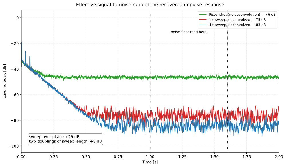
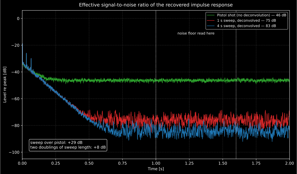
Three recoveries of the same synthetic room impulse response against the same background noise, plotted as smoothed log envelopes against time: a pistol shot recorded directly reaches 46 dB between its peak and the noise floor, a 1 second deconvolved sweep reaches 75 dB, and a 4 second sweep reaches 83 dB, with the floor read in a bracketed window from 1.0 to 1.6 seconds after the room decay has died away

The same room, the same background noise, three excitations. The pistol recovers 46 dB of range; a 1 s deconvolved sweep recovers 75 dB, the 29 dB that clause 6.2.3 predicts. Two further doublings of the sweep add 8 dB — B.6 quotes about 3 dB per doubling as the normal figure, and the extra here is the deconvolution’s own noise tail (B.5) falling away with the longer sweep. The number quoted is the peak-to-floor distance, with the floor read as the RMS of the bracketed window, long after the room has stopped.

Show the code for this figure

import matplotlib.pyplot as plt
import numpy as np
from scipy.signal import fftconvolve
from phonometry import room

fs, n = 48000, 96000
rng = np.random.default_rng(2026)
t = np.arange(n) / fs
system = rng.standard_normal(n) * np.exp(-6.9077 * t / 0.7) * 0.02
system[80] += 1.0; system[1500] += 0.45; system[3200] += 0.28
noise = 10.0 ** (-46.0 / 20.0)          # the room's own background
win = slice(int(1.0 * fs), int(1.6 * fs))

def peak_to_floor(h):
    mag = np.abs(np.asarray(h, dtype=float))
    return 20 * np.log10(mag.max() / np.sqrt(np.mean(mag[win] ** 2)))

shot = system + rng.standard_normal(n) * noise
print(round(peak_to_floor(shot)))                 # 46

for seconds in (1.0, 4.0):
    sweep = room.sweep_signal(fs, 20.0, 20000.0, seconds)
    played = fftconvolve(sweep, system)
    played = played + rng.standard_normal(played.size) * noise
    ir = room.impulse_response(played, sweep, fs, length=n)
    print(seconds, round(peak_to_floor(ir)))      # 1.0 75 / 4.0 83
    plt.plot(t, 20 * np.log10(np.abs(np.asarray(ir)) / np.max(np.abs(np.asarray(ir)))))
plt.show()

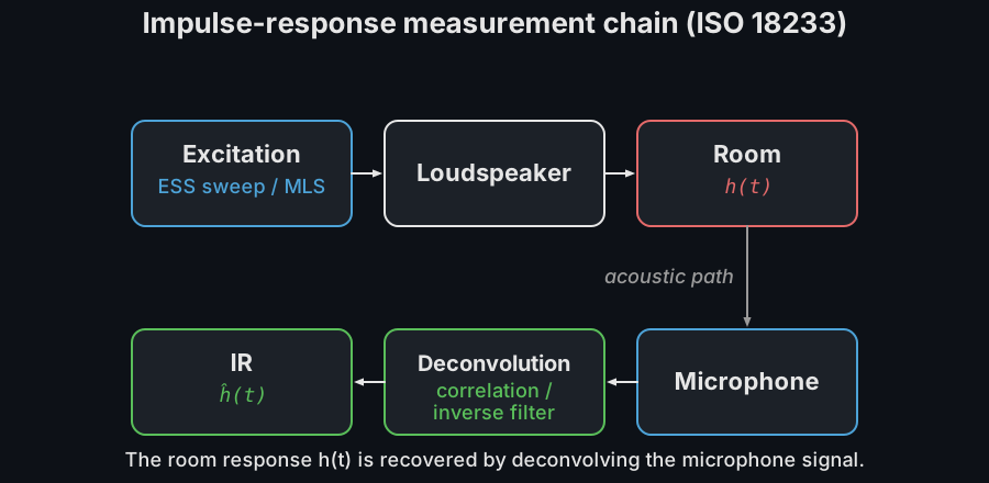
Exponential sine sweep (ESS, Annex B). The instantaneous frequency rises exponentially,

f (t) = f_{1} (\frac{f _{2}}{f _{1}})^{t / T},

so the time spent per octave is constant and the excitation mimics pink noise (constant energy per fractional-octave band). The IR is recovered by linear (zero-padded, non-circular) spectral division,

H = \frac{Y X}{∣ X ∣ ^{2} + ε},

with a small Tikhonov term $ε$ guarding the band edges where the sweep has little energy.

The deconvolution divides by the reference spectrum, so wherever the sweep put no energy there is nothing to divide by, and the Tikhonov term is all that stops the quotient exploding. That is why the sweep starts below the lowest band to be analysed and ends above the highest — typically 20 Hz to 20 kHz for a room analysed from 125 Hz to 4 kHz, since the analysis filters need energy across their skirts as well as at their centres. The symptom of getting it wrong is recognisable: a slow rumble before the direct sound, or a ringing high-frequency tail, either of which lifts the apparent noise floor of the edge bands and shortens their fitted decay times. The rule is to widen the sweep first and raise regularization only when the loudspeaker genuinely cannot reproduce the band — and to record the value used, because it changes the result.

Because a low-to-high sweep places harmonic distortion at negative arrival times, distortion separates cleanly from the linear IR and is discarded by keeping only the causal part. The mechanism is one sentence: the instantaneous frequency of an exponential sweep advances by a fixed number of octaves per second, so the $k$ -th harmonic traces the same frequency path a fixed time earlier, and after deconvolution the distortion collapses into discrete packets at negative delays separated by

Δ t_{k} = T \frac{ln k}{ln ( f _{2} / f _{1} )} .

Three practical consequences follow. The separation is proportional to the sweep length, so a long sweep pushes the packets safely away from $t = 0$ while a very short one lets the second-order packet crowd the linear response. The packets are the raw material of the swept-sine distortion analysis, which is why return_full=True exists. And this separation is why a sweep tolerates a loudspeaker driven near its limit, whereas MLS spreads the same distortion over the whole IR as noise.

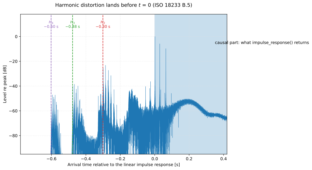
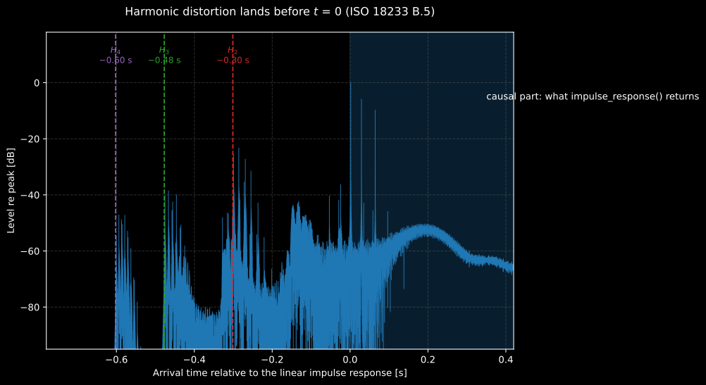
The full deconvolved sequence of a 3 second sweep through a mildly nonlinear chain, plotted on a wrapped time axis with zero in the middle: the linear impulse response at t = 0 with the causal window shaded to its right, and the second, third and fourth harmonic packets as separate clusters at minus 0.30, minus 0.48 and minus 0.60 seconds, each marked with its predicted advance

return_full=True on the same 3 s, 20 Hz to 20 kHz sweep, with a mild memoryless nonlinearity in the chain. The H2, H3 and H4 clusters land at $- Δ t_{k}$ , and the default return simply keeps the shaded half.

Show the code for this figure

import matplotlib.pyplot as plt
import numpy as np
from scipy.signal import fftconvolve
# `room` is the import of the main snippet below.

fs, f1, f2, seconds = 48000, 20.0, 20000.0, 3.0
sweep = room.sweep_signal(fs, f1, f2, seconds)
system = np.zeros(int(0.4 * fs))
system[80], system[1400], system[3100] = 1.0, 0.5, 0.32

played = fftconvolve(sweep, system)
played = played + 0.08 * played ** 2 + 0.04 * played ** 3 + 0.02 * played ** 4
full = np.asarray(room.impulse_response(played, sweep, fs, return_full=True))

for order in (2, 3, 4):
    print(order, round(seconds * np.log(order) / np.log(f2 / f1), 2))
# 2 0.3 / 3 0.48 / 4 0.6   -- the predicted advances, in seconds

half = full.size // 2
plt.plot((np.arange(full.size) - half) / fs,
         20 * np.log10(np.abs(np.roll(full, half)) / np.max(np.abs(full))))
plt.xlim(-0.78, 0.42); plt.ylim(-95, 18)
plt.show()

The "farina" method reaches the same result by convolving the recording with the analytic inverse filter; it assumes the reference sweep was generated with the default amplitude and fade, so use the spectral method for a non-unit-amplitude or custom-fade sweep.

Maximum-length sequence (MLS, Annex A). An order- $N$ binary sequence of length $2^{N} - 1$ whose circular autocorrelation is a near-perfect delta; the IR follows from circular cross-correlation of the recorded period with the sequence. MLS excites at constant amplitude and is quick to average, but it is more sensitive to time variance (draughts, temperature drift) and cannot be fed as much power as a sweep. Prefer the sweep for rooms and partitions; reach for MLS when the excitation must be periodic or the hardware favours a two-level signal.

Dimensioning the excitation

Both excitations are sized against one number the reader already has: the room’s reverberation time $T$ . Get the sizing wrong and nothing looks broken — the result is simply short.

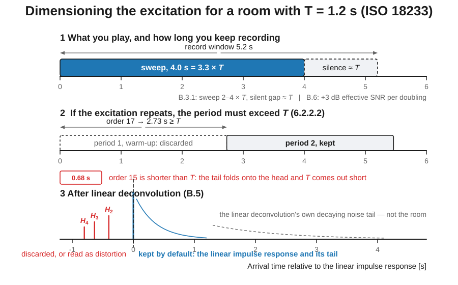
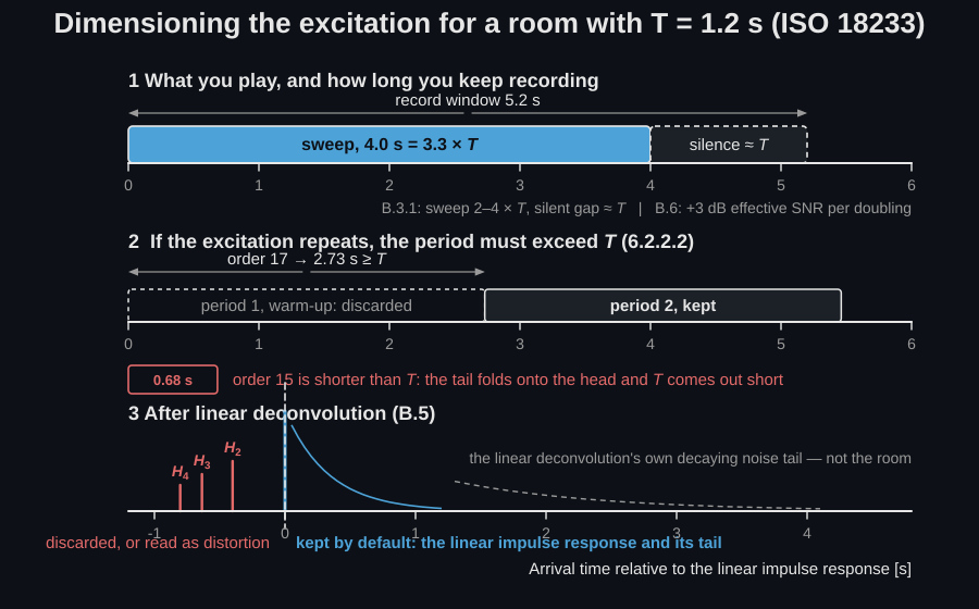
The sweep and its silence. Start the sweep below the lowest analysis band and end it above the highest. Clause B.3.1 calls a length of two to four times the longest expected $T$ , followed by a silent gap of about one $T$ , safe practice under moderate background noise; clause 6.2.2.3 makes the gap normative — the excitation “shall be succeeded by a period of silence”, and the decay shall be recorded over at least half of $T$ . Keep the record running until every band of interest is at least 30 dB down. Then, per B.6, each doubling of the sweep buys about 3 dB of effective SNR, and a longer sweep is preferred over more averages: averaging responses raises the sensitivity to changes in the environment, while one long sweep does not.

The MLS period. A periodic excitation is different, and clause 6.2.2.2 is normative about it (Eq. (10)): the repetition period shall not be shorter than $T$ , so that at least two spectral lines fall inside the bandwidth of any room mode. Since the period of an order- $N$ sequence is $(2^{N} - 1) / f_{s}$ , that fixes the order:

N \geq \frac{l g ( T f _{s} + 1 )}{l g 2} .

At 48 kHz, order 16 gives 1.37 s and order 18 gives 5.46 s, and a room with $T = 1.5$ s needs order 17. Go below that and the tail of one period folds onto the head of the next: the decay is time-aliased, the level floor rises and $T$ comes out short, with no visible symptom. Discard the first period as warm-up, which is what the four-periods-play, three-periods-keep pattern below does.

Three time lanes for a room with T = 1.2 s. The first shows the played sweep of 4.0 seconds, three and a third times T, followed by a silent gap of about one T and a bracketed record window of 5.2 seconds. The second shows a periodic MLS of order 17, period 2.73 seconds, with the first period marked as warm-up and discarded and the second kept, and below it a short order-15 period of 0.68 seconds marked as shorter than T so the tail folds onto the head. The third shows what the deconvolution returns: the linear impulse response and its tail at time zero with the causal part kept, the second, third and fourth harmonic packets at negative arrival times, and the deconvolution's own decaying noise tail

import numpy as np
# `room` is the import of the figure block above.

def excitation_budget(reverberation, fs=48000, factor=3.0):
    """Sweep length, silence and the MLS order a room of this T needs."""
    sweep_seconds = factor * reverberation                   # B.3.1: 2-4 x T
    silence = reverberation                                  # B.3.1: about T
    order = int(np.ceil(np.log2(reverberation * fs + 1.0)))  # 6.2.2.2 Eq. (10)
    period = (2 ** order - 1) / fs
    return round(sweep_seconds, 2), round(silence, 2), order, round(period, 2)

print(excitation_budget(1.2))    # (3.6, 1.2, 16, 1.37)
print(excitation_budget(1.5))    # (4.5, 1.5, 17, 2.73)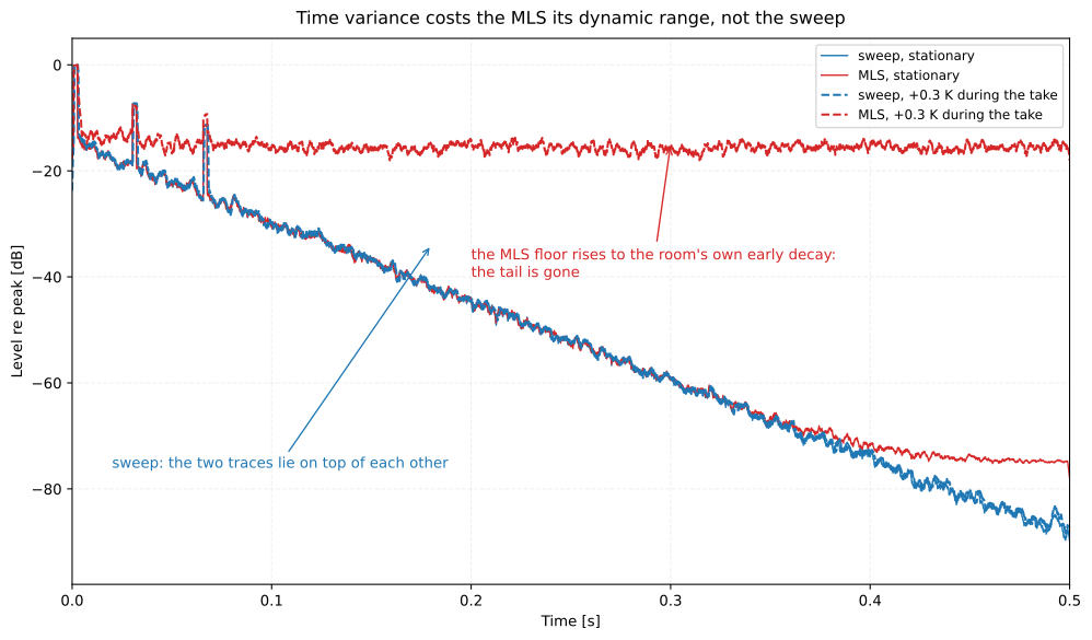

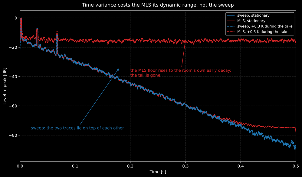
Four recovered impulse-response envelopes from the same synthetic room: the sweep recovered under stationary conditions and under a slow warming of 0.3 kelvin lie on top of each other and reach 90 dB below the peak, the stationary MLS follows them to about 75 dB, and the drifted MLS collapses to a flat floor 15 dB below the peak with no decay left

What “more sensitive to time variance” costs. A slow warming of about 0.3 K across the take — a resampling of 500 parts per million, which is what a falling speed of sound does to the arrival times — leaves the sweep recovery unchanged and destroys the MLS one, because the correlation averages periods that no longer line up. ISO 18233 B.7.3.1 states the same result qualitatively; A.4.3.1 Eq. (A.8) gives the guide limit $Δ ϑ \leq 200/ (f T)$ °C for a reverberation-time measurement.

Show the code for this figure

import matplotlib.pyplot as plt
import numpy as np
from scipy.signal import fftconvolve
# `room` is the import of the main snippet below.

fs, n = 48000, 24000
rng = np.random.default_rng(2026)
t = np.arange(n) / fs
system = rng.standard_normal(n) * np.exp(-6.9077 * t / 0.4) * 0.02
system[80] += 1.0; system[1500] += 0.45; system[3200] += 0.28

def drift(x, ppm):                      # the room warming during the take
    i = np.arange(x.size, dtype=float)
    return np.interp(i, i * (1.0 + ppm * 1e-6 * i / x.size), x, left=0.0, right=0.0)

sweep = room.sweep_signal(fs, 20.0, 20000.0, 1.4)
mls = room.mls_signal(16)
for ppm in (0.0, 500.0):
    played = drift(fftconvolve(sweep, system), ppm)
    plt.plot(20 * np.log10(np.abs(np.asarray(
        room.impulse_response(played, sweep, fs, length=n)))))
    # Four periods played, the first discarded as warm-up. The drifted case
    # trips the library's circular-aliasing warning: that warning IS the result.
    rec = drift(fftconvolve(np.tile(mls, 4), system)[mls.size: 4 * mls.size], ppm)
    plt.plot(20 * np.log10(np.abs(np.asarray(
        room.mls_impulse_response(rec, mls, length=n)))))
plt.show()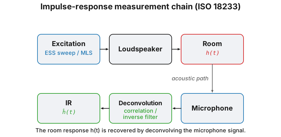

ISO 18233 indirect measurement chain: an ESS sweep or MLS excitation drives a loudspeaker into the room, a microphone captures the response, and deconvolution (correlation or inverse filter) recovers the impulse response

import numpy as np
from scipy.signal import fftconvolve
from phonometry import room

fs = 48000
# A 3 s, 20 Hz - 20 kHz sweep is a good broadband room excitation
# sweep: excitation you play through the loudspeaker
sweep = room.sweep_signal(fs, 20.0, 20000.0, 3.0)

# Deconvolve the recorded response back to the impulse response
system = np.zeros(fs); system[100] = 1.0; system[2000] = 0.4   # direct + reflection
# recorded: mic capture of the played sweep (here simulated by convolution with a synthetic room)
recorded = fftconvolve(sweep, system)
ir = room.impulse_response(recorded, sweep, fs, method="spectral")
print(int(np.argmax(np.abs(ir))))                    # 100: direct sound recovered
ir.plot()                     # waveform + Schroeder envelope (figure below)

# Farina inverse-filter variant (needs the sweep band)
ir_f = room.impulse_response(recorded, sweep, fs, method="farina", f_range=(20.0, 20000.0))

# Periodic MLS: excite with >= 2 periods, average, cross-correlate
mls = room.mls_signal(16)                                 # length 2**16 - 1 = 65535
rec = fftconvolve(np.tile(mls, 2), system)[: 2 * mls.size]
ir_m = room.mls_impulse_response(rec, mls)
print(int(np.argmax(np.abs(ir_m))))                  # 100

sweep_signal/mls_signal return plain arrays, ready to write to a WAV file and play. impulse_response/mls_impulse_response return an ImpulseResponseResult, a drop-in for the raw IR array (np.asarray(ir), indexing and ir.size all keep working, so room_parameters(ir, fs) is unchanged) that also carries the sample rate and method and adds a .plot(). Two more excitations from the transfer-function literature — complementary Golay pairs, whose deconvolution is exact and noise-free, and sweeps shaped to an arbitrary target spectrum — live in the system-measurement guide and return the same result types.

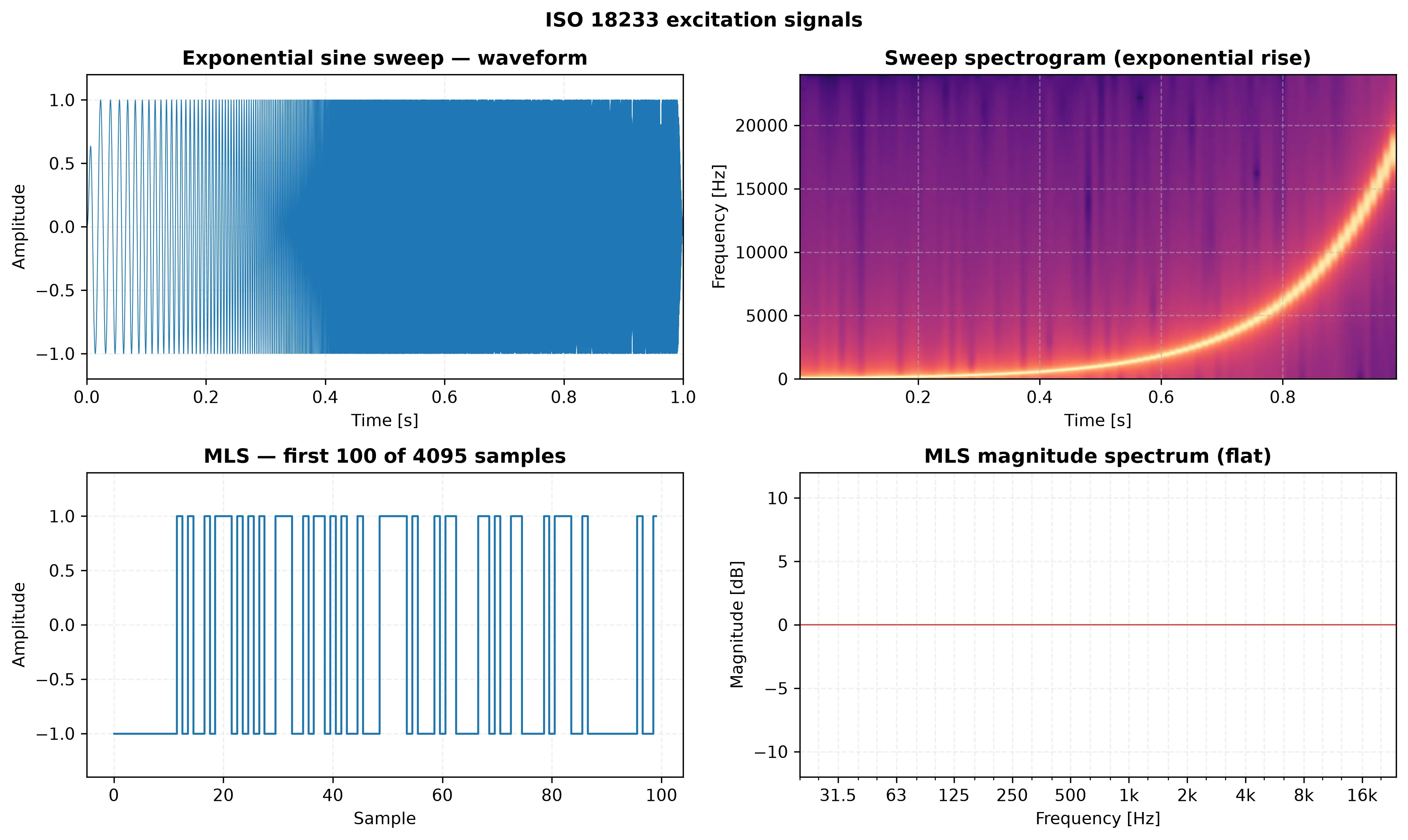
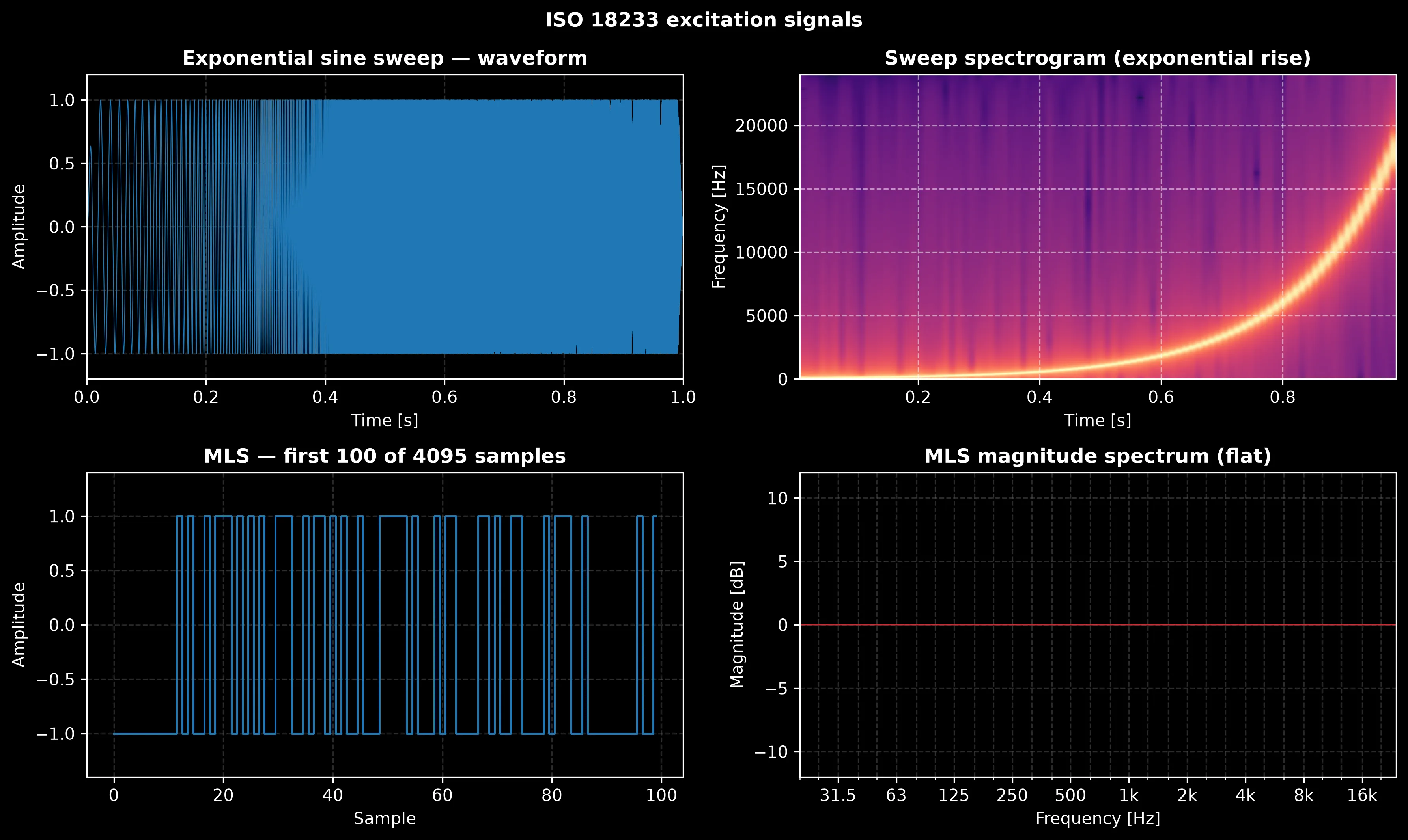
The two excitations. The exponential sweep sweeps its energy up the spectrum over the whole signal, while the MLS is a flat-spectrum two-level sequence, visible as the near-constant magnitude on the right.

ISO 18233 excitation signals: the exponential sine sweep waveform and its spectrogram showing the exponential frequency rise, and a maximum-length sequence with its flat magnitude spectrum

Show the code for this figure

from phonometry import room
from phonometry import plot_excitation

fs = 48000
sweep = room.sweep_signal(fs, 50.0, 20000.0, 1.0)   # ESS excitation
mls = room.mls_signal(12).astype(float)             # length 2**12 - 1

# One-liner: waveform + spectrogram (sweep), sequence + flat spectrum (MLS)
plot_excitation(sweep, fs, kind="sweep")
plot_excitation(mls, fs, kind="mls")

# By hand: the sweep spectrogram and the MLS magnitude spectrum
import numpy as np
import matplotlib.pyplot as plt

fig, (ax1, ax2) = plt.subplots(1, 2, figsize=(12, 4))
ax1.specgram(sweep, NFFT=1024, Fs=fs, noverlap=512)
ax1.set(xlabel="Time [s]", ylabel="Frequency [Hz]", title="Sweep spectrogram")
spec = np.abs(np.fft.rfft(mls))
freqs = np.fft.rfftfreq(mls.size, d=1.0 / fs)
ax2.semilogx(freqs[1:], 20 * np.log10(spec[1:] / np.median(spec[1:])))
ax2.set(xlabel="Frequency [Hz]", ylabel="Magnitude [dB]", title="MLS spectrum (flat)")

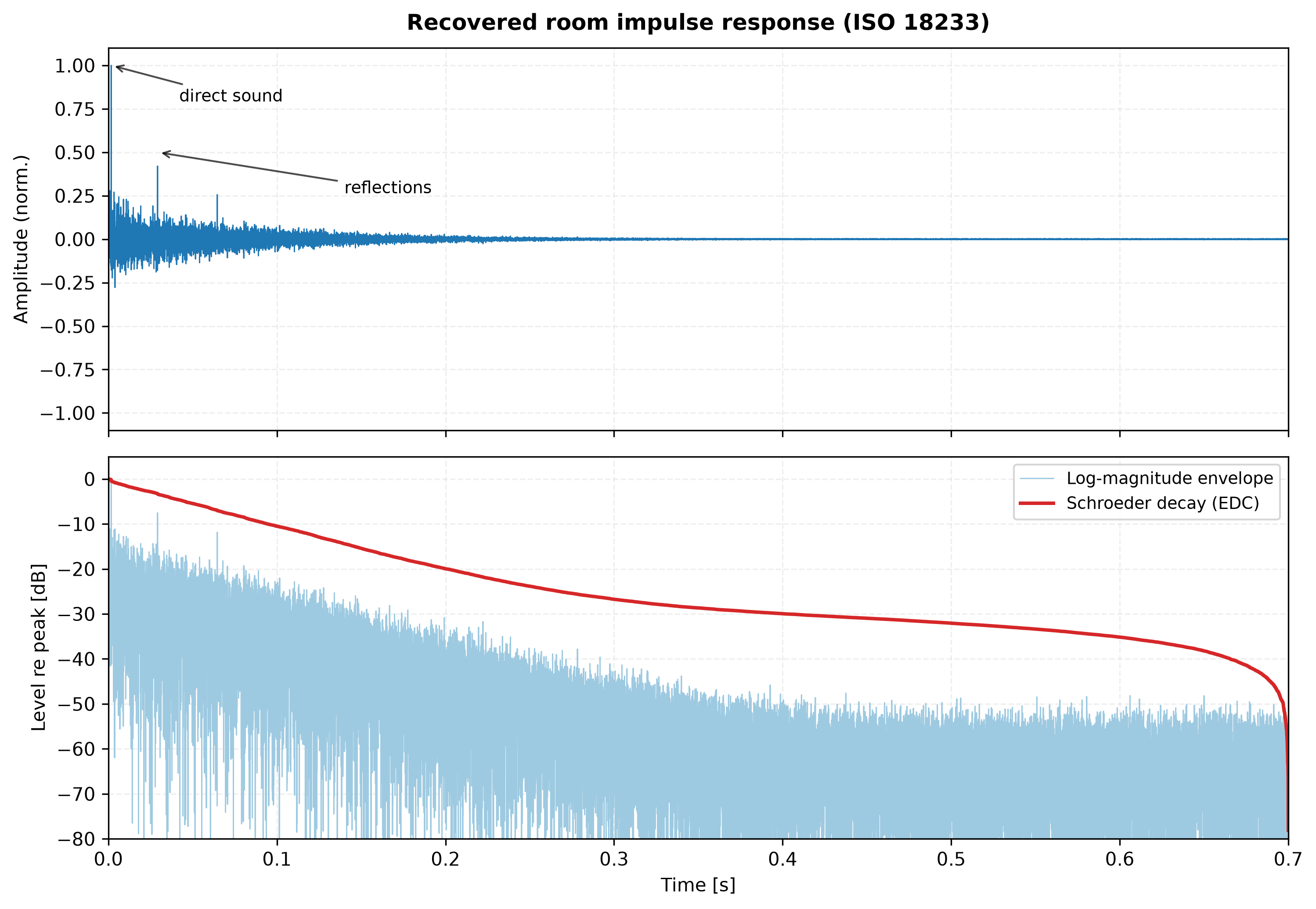
The recovered impulse response

Deconvolving the recording gives the broadband IR: the direct sound, discrete early reflections and the decaying diffuse tail. Its .plot() shows the waveform above and the log-magnitude envelope with the Schroeder energy-decay curve below: the straight decay whose slope becomes the reverberation time in the Room Acoustics guide.

Download the animation (WebM)

Recovered room impulse response: the normalized waveform with the direct sound and reflections labelled, and below it the log-magnitude envelope in dB with the Schroeder energy-decay curve

Show the code for this figure

import numpy as np
from scipy.signal import fftconvolve
# `room` is the import of the main snippet above.

fs = 48000
sweep = room.sweep_signal(fs, 20.0, 20000.0, 1.5)
# A synthetic room: direct sound + two reflections + a decaying diffuse tail
system = np.zeros(int(0.7 * fs))
system[80], system[1400], system[3100] = 1.0, 0.5, 0.32
ir = room.impulse_response(fftconvolve(sweep, system), sweep, fs, length=system.size)

# One-liner: waveform + log-magnitude / Schroeder decay
ir.plot()

# By hand: the normalized log-magnitude envelope in dB
import matplotlib.pyplot as plt
h = np.asarray(ir)
t = np.arange(h.size) / fs
plt.plot(t, 20 * np.log10(np.abs(h) / np.max(np.abs(h))))
plt.ylim(-80, 5)
plt.xlabel("Time [s]"); plt.ylabel("Level re peak [dB]")

One thing this response is not: the impulse response of the room. What the deconvolution returns is the response of loudspeaker, room and microphone in series — clause A.1 of ISO 18233 says as much for the MLS chain, and the sweep is no different. For reverberation time that is harmless, because a fixed linear filter changes the shape of the early part but not the slope of the band decay, which is why reverberation times transfer between measurement systems. For the energy parameters it is not: the source’s low-frequency roll-off and its high-frequency directivity redistribute early energy and shift C50, C80 and $T_{s}$ , so those do not transfer. Two consequences follow. Quote the source used whenever you report clarity or centre time; and remove the free-field response of the chain before auralising the response or comparing it across systems. It is also why the standard specifies the source’s directivity rather than its frequency response: directivity varies between positions and cannot be equalised away.

`sweep_signal()` / `inverse_filter()` parameters

Parameter	Type	Units	Range / default	Notes
`fs`	int	Hz	> 0	Sampling frequency
`f1`	float	Hz	> 0, at/below lowest band	Sweep start frequency
`f2`	float	Hz	`f1 < f2 <= fs/2`	Sweep stop frequency
`seconds`	float	s	2–4 × the longest expected T	Sweep duration; see “Dimensioning the excitation” above
`amplitude`	float	—	default `1.0`	Peak amplitude
`fade`	float	—	`[0, 0.5)`, default `0.01`	Half-Hann fade fraction (kills start/stop transients)

inverse_filter(fs, f1, f2, seconds, amplitude=..., fade=...) takes exactly the same arguments as sweep_signal, because the filter is derived from the sweep it has to invert: it is the time-reversed sweep with a +6 dB/octave envelope, which whitens the ESS’s −3 dB/octave spectrum so that convolving sweep with filter yields an impulse (ISO 18233 B.5). You only call it yourself to inspect the filter or to convolve a recording by hand — impulse_response(..., method="farina") builds it internally from f_range.

`impulse_response()` parameters

Parameter	Type	Units	Range / default	Notes
`recorded`	1D array	any	non-empty	Recorded system response
`reference`	1D array	any	non-empty	The emitted sweep
`fs`	int	Hz	> 0	Sample rate
`method`	str	—	`'spectral'` (default) / `'farina'`	`'farina'` requires `f_range`
`f_range`	(float, float)	Hz	default `None`	`(f1, f2)` of the sweep (Farina only)
`regularization`	float	—	default `1e-6`	Tikhonov term as a fraction of peak spectral energy
`length`	int, optional	samples	default `len(recorded)`	Samples of causal IR to return
`return_full`	bool	—	default `False`	Return the full sequence (distortion in the tail)

mls_signal(order) takes an integer order in 2–20 (sequence length $2^{order} - 1$ ); mls_impulse_response(recorded, mls, length=None) needs recorded to span an integer number of MLS periods.

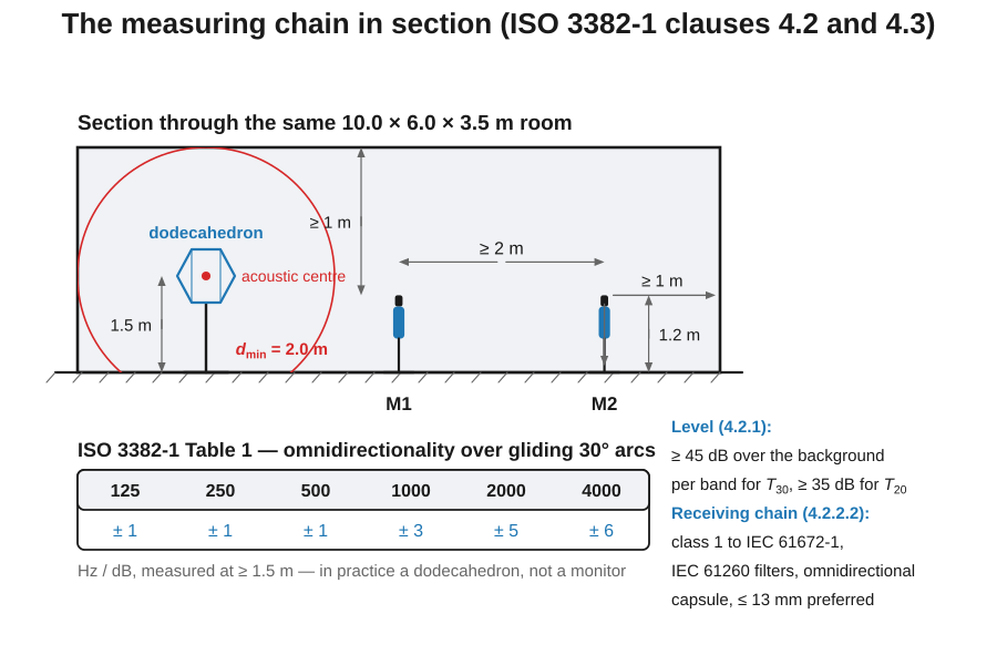
The measuring chain

A deconvolved sweep is only ever as good as what radiated it, and ISO 3382-1 clause 4.2 is specific about all three parts of the chain.

The source (4.2.1). It “shall be as close to omnidirectional as possible”, and Table 1 sets how close, as the maximum deviation from omnidirectionality averaged over gliding 30° arcs in a free field, measured with at least 1.5 m between source and microphone:

Frequency [Hz]	125	250	500	1000	2000	4000
Maximum deviation [dB]	± 1	± 1	± 1	± 3	± 5	± 6

That is why room work uses a dodecahedron and why the output of sweep_signal cannot simply be played through a studio monitor: a one-way monitor is directional well before 1 kHz, and the deviation it would show at 2 and 4 kHz is tens of decibels, not 5 or 6.

The level (4.2.1). Without synchronous averaging, the source must give a level at least 45 dB above the background in the corresponding frequency band if T30 is to be measured, and at least 35 dB if only T20 is needed. The 20–30 dB of processing gain measured at the top of this page is what lets a modest source meet that, but it cannot conjure range in a band where the room is louder than the source. Nothing in the chain may overload (4.2.2.5).

The receiving chain (4.2.2.2). The equipment shall meet the requirements of a type 1 (class 1) sound level meter to IEC 61672-1, with octave or one-third-octave filters to IEC 61260. The microphone shall be omnidirectional and should be as small as possible, preferably with a diaphragm no larger than 13 mm; up to 26 mm is allowed for a pressure- response capsule, or a free-field capsule fitted with a random-incidence corrector.

The heights (4.3). The acoustic centre of the source should be 1.5 m above the floor, at positions where the room’s natural sources would stand, and with at least two source positions. Microphones sit at 1.2 m, seated-ear height, at least a quarter wavelength — “normally around 1 m” — from the nearest reflecting surface including the floor.

Section through a 10 by 6 by 3.5 metre room: a dodecahedron on a stand with its acoustic centre dimensioned 1.5 metres above the floor and its 2.0 metre d_min exclusion circle clipped to the room, two microphones on stands at 1.2 metres with the 2 metre minimum spacing and the 1 metre clearances to the ceiling, the floor and the end wall, and beneath the section the ISO 3382-1 Table 1 omnidirectionality tolerances of plus or minus 1, 1, 1, 3, 5 and 6 decibels from 125 Hz to 4 kHz together with the level and receiving-chain requirements

The same 45 dB is what the T30 validity flag checks downstream: the Room Acoustics guide rejects a band whose decay range does not clear the evaluation window by 15 dB, and that rejection is usually a source-level problem, not a processing one.

Where to measure

One IR characterises a single source–receiver pair; a reported room parameter is the spatial average over several. ISO 3382-1 (performance spaces) asks for at least two source positions and microphones spaced $\geq 2$ m apart, $\geq 1$ m from any surface, at $1.2$ m (seated-ear) height; ISO 3382-2 fixes the minimum number of source, microphone and source–microphone combinations per accuracy grade (survey / engineering / precision) and asks for microphone positions that avoid symmetric placements.

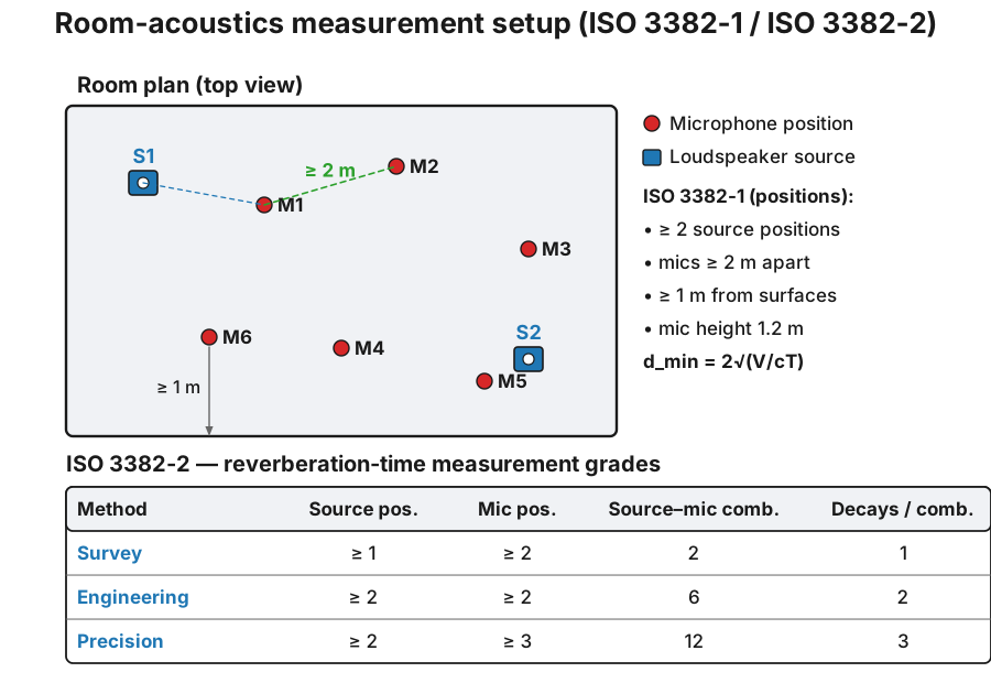
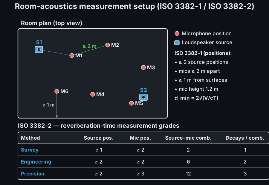
Room-acoustics measurement setup: a top-view room plan with two loudspeaker source positions and six microphone positions with the ISO 3382-1 spacing rules, and the ISO 3382-2 table of minimum positions for the survey, engineering and precision grades

Averaging across positions. The reported per-band parameter is the arithmetic mean over all source-microphone combinations, and the spread across positions is part of the answer, not noise: quote it alongside the mean whenever it exceeds the parameter’s JND (ISO 3382-1 Table A.1), because a room can meet a target on average while individual seats sit far outside it.

Before the four mistakes below, one thing that is not a mistake: a single floor reflection reaching the microphone alongside the direct sound comb-filters the response, and moving the microphone moves the comb with it. That is the mechanism behind the first two mistakes.

Download the animation (WebM)

Four placement mistakes bias the mean itself:

Correlated positions. Microphones closer than 2 m to each other sample nearly the same sound field twice, so the average looks more stable than it is. The 1 m minimum from any surface likewise avoids the pressure build-up near a boundary (the comb filter of the clip above) that colours everything a too-close microphone records.
Symmetric placements. In a geometrically symmetric room, mirror-image positions receive mirror-image reflection patterns; averaging them adds no new information. This is why ISO 3382-2 asks for positions that do not sit on symmetry lines.
Too close to the source. Inside the direct field EDT collapses and C80 saturates upward no matter what the room does. ISO 3382-2 therefore keeps every microphone at least $d_{min} = 2 V / (c \hat{T})$ from the source, with $\hat{T}$ an estimate of the expected reverberation time (2.0 m for the 10 × 6 × 3.5 m room of the drawings above, V = 210 m³, with an expected 0.6 s).
Low-frequency luck. Below the Schroeder frequency (see the Room Acoustics guide) each band holds only a handful of room modes, and a microphone on a node of one of them sees a different decay than a microphone on an antinode. The spread of the 63-125 Hz bands across positions is structurally larger; the cure is more positions, not a longer excitation.

The third mistake is the one worth drawing, because it does not look like a mistake in the result:

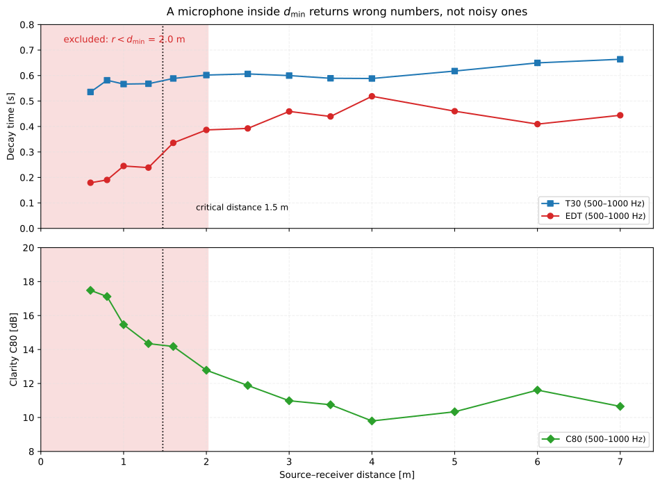
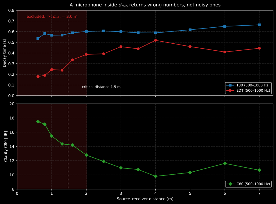
Two stacked panels sharing a source-receiver distance axis from 0.6 to 7 metres in the same 10 by 6 by 3.5 metre room as the setup drawings. Above, the 500 to 1000 Hz mean T30 stays between 0.54 and 0.66 seconds across the whole sweep while EDT climbs from 0.18 to about 0.45 seconds; below, clarity C80 falls from 17.5 to about 10.5 decibels. The region inside d_min = 2.0 metres is shaded as excluded and the critical distance of 1.5 metres is marked with a dotted line

EDT, T30 and C80 of the room above against source distance, from synthetic impulse responses. Inside $d_{min}$ , EDT is short by a factor of about 2.5 and C80 is 7 dB high — many times the 5 % relative and 1 dB just-noticeable differences of ISO 3382-1 Table A.1 — while T30 wanders by 0.12 s over the whole sweep with no trend at the close end. That asymmetry is the trap: a survey that reports only T30 will not notice that the microphone was too close, and every energy parameter beside it is wrong.

Show the code for this figure

import matplotlib.pyplot as plt
import numpy as np
# `room` is the import of the main snippet above.

dims, alpha, source = (10.0, 6.0, 3.5), 0.32, (2.0, 3.0, 1.5)
volume = float(np.prod(dims))
print(round(2.0 * np.sqrt(volume / (343.0 * 0.6)), 1))     # 2.0 m: d_min

for dist in (0.6, 1.0, 2.0, 4.0, 7.0):
    band = []
    for offset in (-0.7, -0.25, 0.25, 0.7):   # one specular receiver scatters
        res = room.image_source_rir(
            dims, source, (2.0 + dist, 3.0 + offset, 1.2), alpha, fs=48000,
            max_order=40,      # c x 0.58 T / L_min, not the default 20
        )
        par = room.room_parameters(res.ir, res.fs, limits=(125.0, 4000.0))
        mid = (par.frequency > 400.0) & (par.frequency < 1200.0)
        band.append([np.mean(par.edt[mid]), np.mean(par.t30[mid]),
                     np.mean(par.c80[mid])])
    print(dist, np.round(np.mean(band, axis=0), 2))
# 0.6 [ 0.18  0.54 17.48]  ...  7.0 [ 0.44  0.66 10.65]
plt.show()

And the fourth is worth counting. The Schroeder frequency is where a room stops being a handful of resonances and starts being a statistical field, and the count is stark:

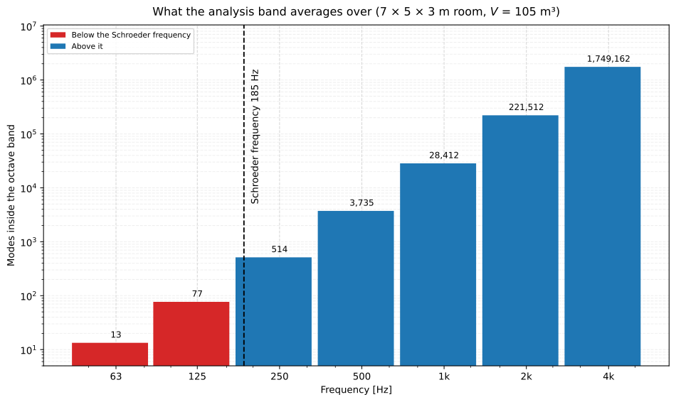
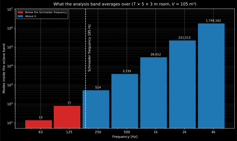
Bar chart on logarithmic axes of the number of room modes inside each octave band from 63 Hz to 4 kHz for a 7 by 5 by 3 metre room of 105 cubic metres: 13 modes at 63 Hz and 77 at 125 Hz, both below the marked Schroeder frequency of 185 Hz, rising to 514 at 250 Hz, 28412 at 1 kHz and 1749162 at 4 kHz

Why “more positions, not a longer excitation”. The 4 kHz octave of this room contains about 1.75 million modes, so the band average does the spatial averaging for you and every microphone reports nearly the same decay. The 63 Hz octave contains 13: which of them a given microphone sits on decides what it measures, and only more microphones can average that out. A longer sweep buys signal-to-noise ratio, which is a different problem.

Show the code for this figure

import matplotlib.pyplot as plt
import numpy as np
# `room` is the import of the main snippet above.

dims, reverberation = (7.0, 5.0, 3.0), 0.9
bands = np.array([63.0, 125.0, 250.0, 500.0, 1000.0, 2000.0, 4000.0])
edge = np.sqrt(2.0)
counts = [room.room_mode_count(f * edge, dims) - room.room_mode_count(f / edge, dims)
          for f in bands]
print([round(c) for c in counts])
# [13, 77, 514, 3735, 28412, 221512, 1749162]
print(round(room.schroeder_frequency(reverberation, float(np.prod(dims)))))   # 185

plt.bar(bands, counts, width=bands * 0.62)
plt.xscale("log"); plt.yscale("log")
plt.show()

The room while you measure it. ISO 3382-2 clause 4.1: reverberation-time measurements “should be made in a room containing no people”, though up to two persons may be present and still represent the unoccupied state unless the specification says otherwise. If the result will be used to correct a level measurement, freeze the occupancy: the same number of people must be present for both. For precision measurements the temperature and relative humidity in the room shall normally be measured — both because the standard requires it and because they set the air-absorption term the prediction guides consume. The exception is stated too: air absorption is negligible when $T$ is shorter than 1.5 s at 2 kHz and 0.8 s at 4 kHz, and then the climate need not be recorded.

The rotating boom. Clause 4.3.1 allows a moving microphone in place of discrete positions, with three constraints: a sweep radius of at least 0.7 m, a traverse plane at least 10° off every plane of the room (wall, floor, ceiling), and a traverse period of at least 15 s. It substitutes for multiple microphone positions only where the Table 1 grade allows it — for the interrupted-noise method, and where the result is a correction term.

What the report must carry (clause 9.2). A statement of conformity with ISO 3382-2; enough to identify the room uniquely; a scaled sketch plan; the volume; the condition of the room (furniture, people present); for the precision method, the temperature and relative humidity; the type of source and a description of the signal; the degree of precision — survey, engineering or precision — with the source and microphone positions, preferably shown on that plan together with their heights; the measuring apparatus and microphones; the evaluation method for the decay curves; how the result was averaged in each position and over positions; the results table; and the date and the measuring organisation. The fiche of the Room Acoustics guide carries most of these as ReportMetadata fields, but the scaled plan with the positions on it has to be supplied alongside it.

From the impulse response onward

The IR leaves this page in several directions. Band-filtered and backward-integrated it becomes the decay curve whose slope is the reverberation time: the Room Acoustics guide picks up exactly there, and its open-plan sibling walks the ISO 3382-3 line of workstations. Measured either side of a partition, the same sweeps feed the level differences of field sound insulation. And the harmonic distortion that the exponential sweep pushes to negative arrival times is not always discarded: read deliberately, it becomes the THD analysis of the swept-sine distortion guide.

What this guide covers

Covered
ISO 18233:2006’s deterministic acquisition of the room impulse response: the Annex B exponential sine sweep (room.sweep_signal, room.inverse_filter) with linear spectral deconvolution (Tikhonov-regularized) and the Farina inverse-filter variant (room.impulse_response, methods "spectral" and "farina"), and the Annex A maximum-length sequences (room.mls_signal, orders 2-20, room.mls_impulse_response by circular cross-correlation). The results are ImpulseResponseResult objects that drop into room.room_parameters unchanged. The ISO 18233 sizing rules (clause B.3.1 sweep length and silence, clause 6.2.2.2 Eq. (10) for the MLS period), the ISO 3382-1 clause 4.2 equipment requirements and the ISO 3382-1/-2 placement rules (spacing, surface distance, the minimum source distance, the rotating-boom alternative and the accuracy grades) are quoted for planning, together with the clause 9.2 report checklist.
Not covered
Playback and recording themselves (sound-card I/O, level calibration of the chain) are outside the library. ISO 18233’s time-variance and distortion diagnostics are not implemented: the guide explains how the sweep separates distortion, but no helper quantifies it (that reading lives in the swept-sine distortion guide). The position rules are guidance prose: nothing checks how many positions were measured or where.

Quick answers

Should I measure the room impulse response with a sine sweep or an MLS?

Both are ISO 18233 deconvolution methods that recover the impulse response with 20–30 dB more effective signal-to-noise ratio than an impulsive source. Prefer the exponential sine sweep (Annex B): it places harmonic distortion at negative arrival times, where it is discarded. Use MLS (Annex A) when the excitation must be periodic or the hardware favours a two-level signal; it is more sensitive to time variance.

References

International Organization for Standardization. (2006). Acoustics — Application of new measurement methods in building and room acoustics (ISO 18233:2006). The swept-sine and MLS acquisition this page implements.
International Organization for Standardization. (2008). Acoustics — Measurement of room acoustic parameters — Part 2: Reverberation time in ordinary rooms (ISO 3382-2:2008). The accuracy grades, position counts and the minimum source distance behind the position-averaging discussion.
International Organization for Standardization. (2009). Acoustics — Measurement of room acoustic parameters — Part 1: Performance spaces (ISO 3382-1:2009). The source and microphone position requirements quoted in the where-to-measure rules.

Created and maintained by José Manuel Requena Plens ORCID All projects

Measuring the Room Impulse Response

Two deterministic excitations (ISO 18233)

Dimensioning the excitation

The recovered impulse response

sweep_signal() / inverse_filter() parameters

impulse_response() parameters

The measuring chain

Where to measure

From the impulse response onward

What this guide covers

See also

Quick answers

Should I measure the room impulse response with a sine sweep or an MLS?

References

`sweep_signal()` / `inverse_filter()` parameters

`impulse_response()` parameters