Sound absorption in enclosed spaces (EN 12354-6)

EN 12354-6:2003 predicts the total equivalent sound absorption area of a room and its reverberation time from the absorption of its surfaces and objects, the design counterpart of the measured reverberation time. It is the absorption member of the EN 12354 building-acoustics family (the airborne and impact insulation members live in Predicting Sound Insulation (EN 12354)). phonometry implements the normative Clause 4 model. (The informative Annex D method for irregular spaces is out of scope.)

That family membership is the reason most acousticians run this calculation. The equivalent absorption area $A$ is not only an end in itself: it is the quantity that converts an insulation prediction into a rated one. A prediction produces a level difference $D$, and the ratings are defined only once the receiving room’s absorption is known — $D_{nT}=D+10\lg (T/T_0)$ and $R^{\prime }=D+10\lg (S/A)$ — while EN 12354-5 needs the same $A$ to turn a service installation’s sound power into a room level. The direction of the error matters: over-estimating the receiving room’s absorption flatters the predicted $D_{nT}$, so the same optimistic ${\alpha }_s$ data that shortens the predicted reverberation time also inflates the predicted insulation rating. That is why the standard insists the source of every coefficient be stated in the report.

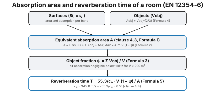
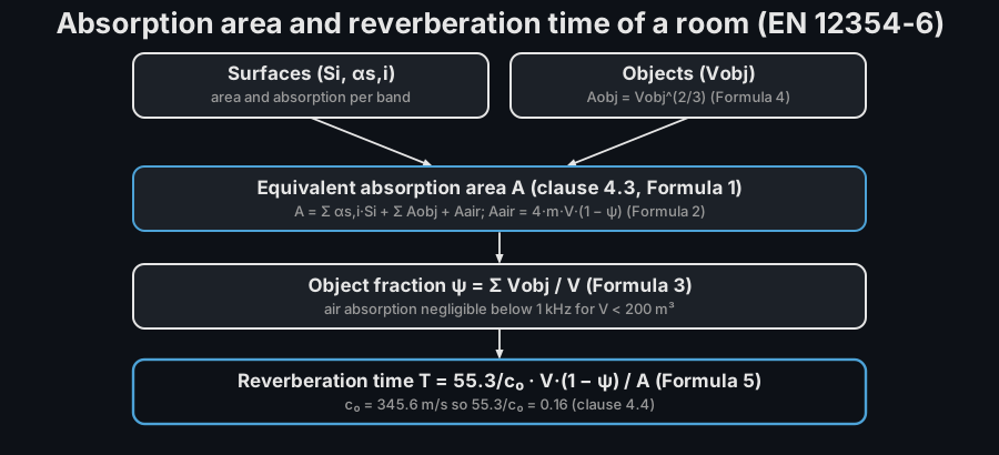
1. Equivalent absorption area (clause 4.3)

The total equivalent absorption area sums, over the surfaces $i$, the objects $j$ and the object arrays $k$, each surface’s area times its absorption coefficient, the equivalent absorption areas of the objects, the object arrays (groups of identical objects treated as an absorbing surface of area $S_k$), and the air absorption (Formula 1):

$$A=\sum _i{\alpha }_{s,i}{S}_i+\sum _j{A}_{\mathrm{obj},j}+\sum _k{\alpha }_{s,k}{S}_k+A_{\mathrm{air}}.$$

For hard, irregular objects whose absorption is not measured, an empirical estimate from the volume is used (Formula 4): $A_{\mathrm{obj}}=V_{\mathrm{obj}}^{2/3}$. The exponent is a surface-area scaling: an object’s exposed area grows as the two-thirds power of its volume, so the formula credits a hard object with roughly one face of its bounding cube of perfectly absorbing surface. It is frequency-independent by construction, which is why it is restricted to hard, irregular objects — anything soft, resonant or tabulated needs a measured $A_{\mathrm{obj}}$ instead — and why clause 4.5 adds that objects matter only when they are large compared with the wavelength, so anything under about 1 m across can normally be left out.

The take-off itself is the half of the calculation a drawing does not hand you. The diagram below turns EN 12354-6’s own Annex E room into the three input lists the formulae consume, so each number in the snippet that follows has a surface behind it.

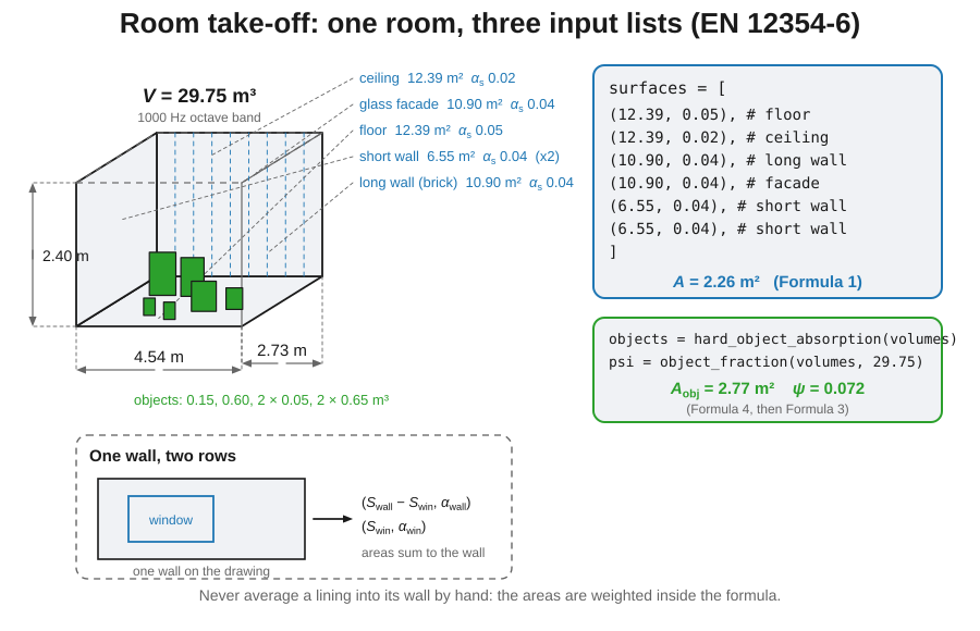
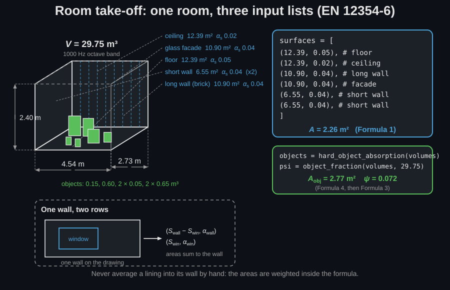
The Annex E room at 1 kHz, taken off surface by surface. Every row of the surfaces list below is one tagged boundary; the furniture becomes the objects list through Formula 4, and its summed volume becomes $\psi$. The inset is the rule that governs every real room: a wall carrying a window is two rows whose areas sum to the wall, never one row with an averaged coefficient.

from phonometry import room

# EN 12354-6 Annex E, bare room (29.75 m3), 1000 Hz octave band.
# The six rows are floor, ceiling, long wall, glass facade and the two
# short walls of a 4.54 x 2.73 x 2.40 m room.
surfaces = [(12.39, 0.05), (12.39, 0.02), (10.90, 0.04),
            (10.90, 0.04), (6.55, 0.04), (6.55, 0.04)]
print(round(room.equivalent_absorption_area(surfaces), 2))  # 2.26  m2
print(round(float(room.hard_object_absorption(0.65)), 3))   # 0.75  m2

Air absorption uses the power attenuation coefficient $m$ (Formula 2): $A_{\mathrm{air}}=4mV(1-\psi )$. Below 1 kHz and for rooms under 200 m³ it can be neglected.

2. Reverberation time (clause 4.4)

The reverberation time follows from the absorption area, the volume and the object fraction $\psi =\sum V_{\mathrm{obj}}/V$ (Formula 5):

$$T=\frac{55.3}{c_0}\frac{V(1-\psi )}{A},$$

where the speed of sound $c_0=345.6\text{m/s}$ makes the factor $55.3/c_0$ the familiar $0.16$.

The 55.3 is $24\ln 10=55.262$, the constant that falls out of the diffuse-field decay when the mean free path is $4V/S$ and the decay is extrapolated to a full 60 dB (the classical derivation). Formula 5 is therefore Sabine’s law applied to the free volume left after the objects have displaced their share, and the standard’s unusual $c_0$ is a rounding convention rather than a claim about the air temperature: 345.6 m/s is chosen precisely so the quotient is the traditional 0.16. The residue is small but real — for the same room this returns times about 0.7 % shorter than sabine_reverberation_time at its own $c_0=343$ m/s.

from phonometry import room

surfaces = [(12.39, 0.05), (12.39, 0.02), (10.90, 0.04),
            (10.90, 0.04), (6.55, 0.04), (6.55, 0.04)]
a = room.equivalent_absorption_area(surfaces)
print(round(room.reverberation_time(a, 29.75), 1))          # 2.1  s

# Annex E case 2: add furniture (hard objects) to the same room.
volumes = [0.15, 0.60, 0.05, 0.05, 0.65, 0.65]
aobj = room.hard_object_absorption(volumes)
psi = room.object_fraction(volumes, 29.75)                  # 0.072
a2 = room.equivalent_absorption_area(surfaces, objects=aobj)
print(round(a2, 2), round(room.reverberation_time(a2, 29.75, object_fraction=psi), 1))
# 5.03 0.9

Both numbers are worth reading rather than passing over. A bare 30 m³ room at 2.1 s is unusable for speech — well over three times any classroom target — and six pieces of hard furniture then supply 2.77 m² of absorption against the 2.26 m² of all six room surfaces together, more than doubling $A$ and halving $T$. Almost all of that comes from the objects’ own absorption; the $\psi$ term contributes only the last 7 %, as the right-hand panel below separates out.

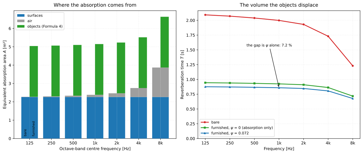
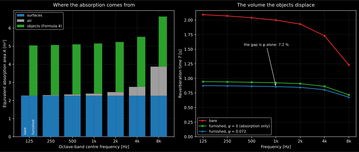
The Annex E pair, per octave band. The objects add a flat, frequency-independent 2.77 m² (Formula 4 has no frequency in it), which is why the furnished bars gain the same absolute height in every band and the relative improvement is largest where the room was deadest to begin with. On the right, the gap between the two furnished curves is the whole effect of the displaced volume: $\psi$ = 0.072 removes 7.2 % of the free volume and so shortens $T$ by 7.2 %, an order of magnitude less than the objects’ absorption does.

Show the code for this figure

import matplotlib.pyplot as plt
import numpy as np
# `room` is the import of the Annex E block above.

bands = [125.0, 250.0, 500.0, 1000.0, 2000.0, 4000.0, 8000.0]
alpha = {"floor": 0.05, "ceiling": 0.02, "wall": 0.04}   # 1 kHz, held per band
per_band = [(12.39, [alpha["floor"]] * 7), (12.39, [alpha["ceiling"]] * 7),
            (10.90, [alpha["wall"]] * 7), (10.90, [alpha["wall"]] * 7),
            (6.55, [alpha["wall"]] * 7), (6.55, [alpha["wall"]] * 7)]
volumes = [0.15, 0.60, 0.05, 0.05, 0.65, 0.65]
bare = room.enclosed_space_reverberation(per_band, 29.75, air_condition="20C_50-70")
furnished = room.enclosed_space_reverberation(
    per_band, 29.75, objects=room.hard_object_absorption(volumes),
    object_fraction=room.object_fraction(volumes, 29.75),
    air_condition="20C_50-70",
)

fig, (left, right) = plt.subplots(1, 2, figsize=(12.5, 5.0))
x = np.arange(len(bands))
left.bar(x - 0.2, bare.absorption_area, 0.4, label="bare")
left.bar(x + 0.2, furnished.absorption_area, 0.4, label="furnished")
left.set_ylabel(r"$A$ [m$^2$]")
left.legend()
right.semilogx(bands, bare.reverberation_time, label="bare")
right.semilogx(bands, furnished.reverberation_time, label=r"furnished, $\psi$ = 0.072")
right.set_ylabel(r"$T$ [s]")
right.legend()
plt.show()

Per octave band, one call takes the surfaces (with per-band absorption coefficients) and the air condition and returns the whole spectrum:

from phonometry import room

# Per-band absorption coefficients (125 Hz to 8 kHz) for each surface.
plaster = [0.02, 0.03, 0.03, 0.04, 0.05, 0.05, 0.05]
tile = [0.15, 0.35, 0.65, 0.85, 0.90, 0.90, 0.85]
result = room.enclosed_space_reverberation(
    [(54.0, plaster), (20.0, plaster), (20.0, tile)],
    volume=60.0, air_condition="20C_50-70",
)
print(result.reverberation_time.round(2))
# [2.13 1.03 0.62 0.48 0.43 0.42 0.4 ]
result.plot()   # A and T per octave band, for this room alone

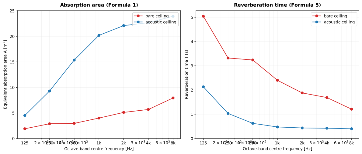
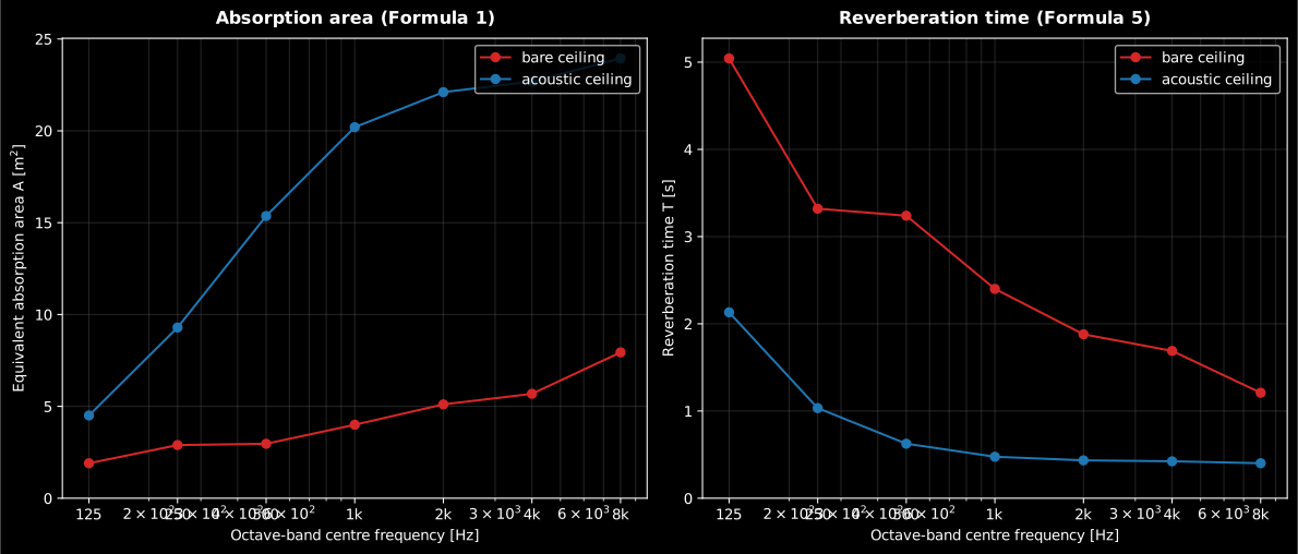
The figure below runs that call twice, once with the acoustic tile above and once with the ceiling left as bare plaster, so the treatment can be read off as a difference. The [2.13 1.03 …] printed above is its “acoustic ceiling” curve; result.plot() draws that curve on its own.

Show the code for this figure

import matplotlib.pyplot as plt
from phonometry import room

plaster = [0.02, 0.03, 0.03, 0.04, 0.05, 0.05, 0.05]
tile = [0.15, 0.35, 0.65, 0.85, 0.90, 0.90, 0.85]
walls_floor = [(54.0, plaster), (20.0, plaster)]
for ceiling in (plaster, tile):
    room.enclosed_space_reverberation(
        [*walls_floor, (20.0, ceiling)], 60.0, air_condition="20C_50-70",
    ).plot()
plt.show()

The same 60 m³ office with two ceilings. Swapping 20 m² of plaster for acoustic tile multiplies the equivalent absorption area by 4 to 5 above 500 Hz (4.0 m² to 20.2 m² at 1 kHz) and pulls the reverberation time from 2.4 s to 0.48 s there. The 125 Hz band, where the tile is weakest, improves least — 1.9 m² to 4.5 m², and 5.04 s only down to 2.13 s: a 20 mm porous tile is a small fraction of a 2.7 m wavelength and absorbs by friction only where the particle velocity is high, so low-frequency control needs depth, an air gap or a resonant absorber.

The ReverberationResult carries the per-band absorption area and reverberation time, the volume and the object fraction, and its .plot() draws the reverberation-time spectrum. This is the prediction counterpart of the measured reverberation time in Room Acoustics (ISO 3382) and of the reverberation-room absorption of Sound Absorption Measurement and Rating (ISO 354).

2b. Designing to a target

EN 12354-6 exists to support design, and design runs the formulae backwards: from a target reverberation time to the absorption area the room must have, to the deficit against the untreated room, to the area of a chosen product. Inverting Formula 5 gives

$$A_{\text{required}}=\frac{55.3}{c_0}\frac{V(1-\psi )}{T_{\text{target}}}=\frac{0.16V(1-\psi )}{T_{\text{target}}},$$

which has to be evaluated band by band, because the target is normally a range across 125 Hz to 4 kHz rather than a single number. Subtract the absorption the untreated room already has to get the per-band deficit, divide the deficit by the candidate product’s per-band ${\alpha }_s$ to get the area to install, and then check that area actually fits on the available surfaces.

import numpy as np
# `room`, `plaster` and `tile` come from the per-band block above.

bare = room.enclosed_space_reverberation(
    [(54.0, plaster), (20.0, plaster), (20.0, plaster)],
    volume=60.0, air_condition="20C_50-70",
)
required = 0.16 * 60.0 / 0.6                     # 16.0 m2 for a 0.6 s target
deficit = required - bare.absorption_area
print(np.round(deficit, 1))                      # [14.1 13.1 13.  12.  10.9 10.3  8.1]
print(np.round(deficit / np.array(tile), 0))     # [94. 37. 20. 14. 12. 11.  9.] m2 of tile

The answer is the design lesson. Above 500 Hz the target needs about 20 m² of tile, which is exactly the ceiling area, and the treated room of §2 duly lands at 0.48 s. At 125 Hz it would need 94 m² — the room’s entire boundary — so the target is simply unreachable with a thin porous product, which is the general rule: the deficit is largest at 125 Hz where such products are weakest. Two consequences follow from the model itself. Because the reverberant level falls as $10\lg A$, doubling the absorption area buys only 3 dB, so a room a second over target cannot be rescued with a rug. And because $A$ appears in the denominator, the first square metres of treatment are worth far more than the last: going from 2 m² to 6 m² of absorption thirds the reverberation time, while going from 20 m² to 24 m² changes it by a sixth.

Anchors for the target itself, since the standard supplies none: speech-critical rooms such as classrooms and meeting rooms usually sit between about 0.4 s and 0.8 s at mid frequencies depending on volume, with ANSI/ASA S12.60-1:2010 Table 1 capping unoccupied, furnished core learning spaces at 0.6 s up to 283 m³ and 0.7 s from 283 m³ to 566 m³; open offices, corridors and stairwells are specified by absorption area rather than by reverberation time, which is clause 4.5’s own advice (§3); and music spaces need longer times than this standard is intended for. The classical prediction guide carries the same anchors with their frequency-shape rules.

3. Where the input data comes from

Surface coefficients. The standard expects the ${\alpha }_{s,i}$ to come from laboratory measurements to EN ISO 354, the reverberation-room method of Sound Absorption Measurement and Rating; theoretical, empirical or field values are admitted as long as the data source is stated. ISO 354 delivers one-third-octave data, and an octave-band calculation takes the arithmetic mean of the three thirds as its input. A reverberation-room coefficient can exceed 1.0 (edge diffraction scatters more energy into the sample than its flat area intercepts); it enters Formula 1 as measured, without clamping, because the same diffuse-field convention that produced it is the one the model assumes.

Not the single-number rating. The standard admits frequency-band data only. Clause 3.2.1’s NOTE is explicit that a single-number rating derived per EN ISO 11654 — ${\alpha }_w$, and by the same argument the NRC and SAA of the American practice — may be used for comparing or specifying products but cannot be used directly to calculate the performance in situ. This is the commonest way to get the calculation wrong, and it runs silently, because the API accepts a scalar coefficient per surface and will happily apply a datasheet’s headline figure to every band. Three properties of the rating make that substitution wrong in a known direction. It is a shifted reference curve read at 500 Hz, fitted by moving the curve in 0.05 steps until the summed unfavourable deviations fall to 0.10 or less, so a band that under-performs is absorbed into that allowance rather than reported. Its inputs, the practical coefficients ${\alpha }_p$, are already rounded in steps of 0.05 and capped at 1.00. And its reference curve stops at the 250 Hz octave, so ISO 11654 states that the rating is not appropriate below that frequency at all: a flat ${\alpha }_w$ carries no information whatsoever about the 125 Hz band, which is where rooms usually fail. Compare the 20 mm tile of §2, whose ${\alpha }_s$ runs 0.15 at 125 Hz against 0.85 at 1 kHz, with the single “Class A” figure its datasheet would print. Take the per-third-octave table from the ISO 354 test report and average the three thirds into each octave; where only a rating is available, treat the prediction as indicative and say so in the report. The rating itself is defined in Sound Absorption Measurement and Rating.

Furniture and occupants. Objects contribute through three routes: a measured equivalent absorption area $A_{obj}$ when one exists (persons and seating have tabulated values in the informative Annex C), the Formula 4 estimate $V_{obj}^{2/3}$ for hard, irregular, unmeasured objects (furniture, machinery), and object arrays rated as an absorbing surface ${\alpha }_s{S}_k$ when many similar objects cover a zone (an audience, a storage rack). Objects also displace air: their summed volume enters the object fraction $\psi$ that shortens $T$ in Formula 5 beyond what their absorption alone would.

Air. The air term $A_{air}=4mV(1-\psi )$ uses the power attenuation coefficient $m$ from the standard’s Table 1, resolved by the air_condition strings (temperature and relative-humidity class, derived from ISO 9613-1); it only matters above 1 kHz and grows with the volume. The six built-in profiles, "10C_30-50" through "20C_70-90" (clause 4.3 recommends "20C_50-70" when no conditions are specified), cover the standard 125 Hz to 8 kHz octave bands only and cannot be combined with a custom frequency axis; air_condition=None (the default) omits the air term, and for other frequencies or conditions compute $m$ per ISO 9613-1 and chain air_absorption_area into equivalent_absorption_area.

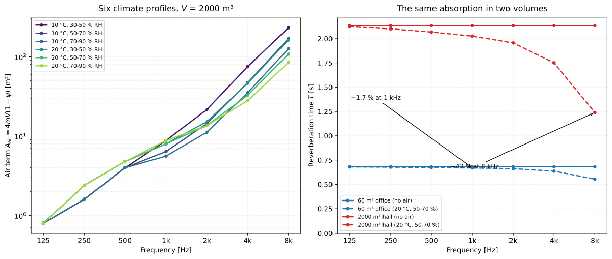
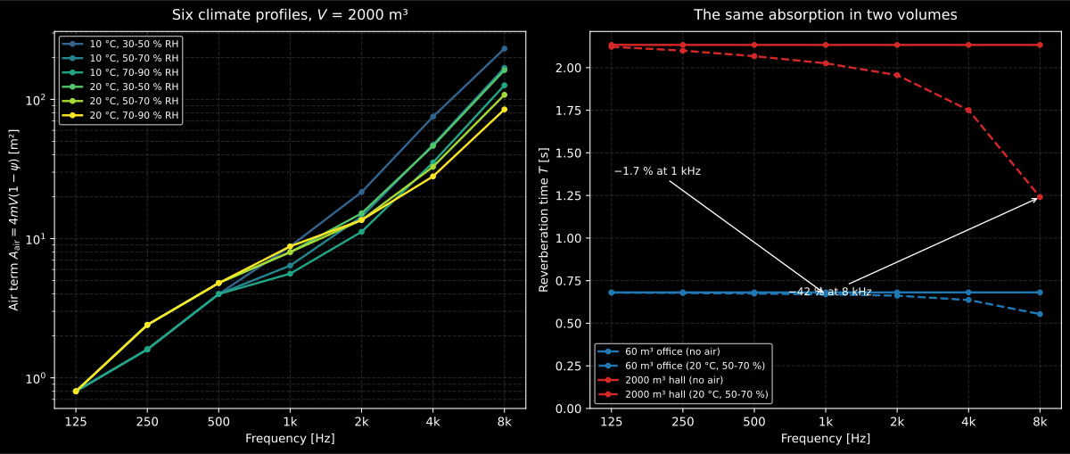
Left: the air term for the six built-in profiles at a fixed 2000 m³. EN 12354-6 Table 1 gives the same 0.1 × 10⁻³ Np/m at 125 Hz for every climate, so the six curves are indistinguishable there; by 8 kHz they run from 10.6 to 29.0 × 10⁻³ Np/m, a factor of 2.7, with the cold, dry profile absorbing most. Right: the same $\bar{\alpha }$ = 0.15 in two volumes, showing what the thresholds in the prose are worth. In the 60 m³ office the air term costs 1.7 % at 1 kHz and is still under 3 % at 2 kHz; in the 2000 m³ hall it costs 5.1 % at 1 kHz, 18 % at 4 kHz and 42 % at 8 kHz. The volume threshold and the frequency threshold are one rule, not two: the term is $4mV$ against a boundary term that grows only as the area.

Show the code for this figure

import matplotlib.pyplot as plt
# `room` is the import of the per-band block above.

bands = [125.0, 250.0, 500.0, 1000.0, 2000.0, 4000.0, 8000.0]
profiles = ["10C_30-50", "10C_50-70", "10C_70-90",
            "20C_30-50", "20C_50-70", "20C_70-90"]
soft = [0.15] * 7

# The air term is the difference the air_condition string makes to A.
fig, (left, right) = plt.subplots(1, 2, figsize=(12.5, 5.0))
still = room.enclosed_space_reverberation([(1000.0, soft)], 2000.0)
for name in profiles:
    humid = room.enclosed_space_reverberation(
        [(1000.0, soft)], 2000.0, air_condition=name)
    left.loglog(bands, humid.absorption_area - still.absorption_area,
                marker="o", label=name)
left.set_ylabel(r"$A_{air}$ [m$^2$]")
left.legend(fontsize=8)

for volume, area in ((60.0, 94.0), (2000.0, 1000.0)):
    for condition in (None, "20C_50-70"):
        res = room.enclosed_space_reverberation(
            [(area, soft)], volume, air_condition=condition)
        right.semilogx(bands, res.reverberation_time,
                       label=f"{volume:g} m3, air={condition}")
right.set_ylabel(r"$T$ [s]")
right.legend(fontsize=8)
plt.show()

Validity limits (clause 4.6). The model assumes an ordinary, reasonably diffuse room: no dimension more than 5 times another, opposite surface pairs whose coefficients differ by less than a factor of 3 (unless scattering objects are present) and an object fraction below 0.2. Outside those limits the field is not diffuse and the model errs on the optimistic side: the standard’s own accuracy clause records measured reverberation times up to twice the prediction in low-diffusivity rooms. The classical alternatives for those cases live in Reverberation-time prediction.

Two scope statements sit above those numeric limits. Clause 1 says the model is based on experience with rooms in dwellings and offices and with common spaces such as stairwells, corridors and rooms containing machinery, and that it is not intended for very large or irregularly shaped spaces such as concert halls, theatres and factories — for which the room-acoustic measurement standards and the classical formulae are the right tools. And clause 4.1 fixes the normal calculation range at the 125 Hz to 4 kHz octaves, with a NOTE recording that no accuracy information exists outside it; the air table and this implementation extend to 8 kHz, so treat that band as an extrapolation. Annex E supplies a worked demonstration that the limits bite: its own case 3, a single wall lined over 90 % of its area, is declared to be outside the application limits of the model, and the annex hands the case to the informative Annex D method instead.

Reading the numbers (clause 4.5). The standard’s own interpretations turn three of the quantities on this page into judgements:

• Objects smaller than about 1 m across can normally be neglected, because they only matter when their dimensions exceed the wavelength.
• An empty room typically has $\psi <0.05$ and a furnished one $0.05\le \psi \le 0.2$, which places the Annex E value of 0.072 squarely in the ordinary furnished range. A $\psi$ far above that band signals a plant room whose remaining free space may no longer behave as a single space at all, which is a scope question rather than an accuracy one.
• In a stairwell, an entrance hall or a plant room the reverberation time is a poor descriptor and the requirement is better written as an amount of absorption — which is why equivalent_absorption_area is exposed independently of reverberation_time rather than only as an intermediate.

Estimating the accuracy (clause 5). The standard declines to state an accuracy and gives one piece of practical advice instead: vary the input data, especially in complicated situations and with atypical elements, and read the resulting spread as the expected accuracy.

# `room`, `plaster` and `tile` come from the per-band block above.
for factor in (0.8, 1.0, 1.2):                 # the ceiling alpha, plus or minus 20 %
    ceiling = [a * factor for a in tile]
    res = room.enclosed_space_reverberation(
        [(54.0, plaster), (20.0, plaster), (20.0, ceiling)],
        volume=60.0, air_condition="20C_50-70",
    )
    print(factor, res.reverberation_time.round(2))
# 0.8 [2.46 1.22 0.75 0.57 0.52 0.5  0.47]
# 1.0 [2.13 1.03 0.62 0.48 0.43 0.42 0.4 ]
# 1.2 [1.88 0.9  0.53 0.41 0.37 0.37 0.35]

A ±20 % uncertainty on one surface’s coefficient moves the 1 kHz prediction from 0.48 s to 0.57 s or 0.41 s — +19 % and −15 %, asymmetric because $T$ goes as $1/A$ — and 2.13 s to 2.46 s or 1.88 s at 125 Hz, where the ceiling carries less of the total. That spread is the accuracy statement the standard declines to give, so a design that clears its target by less than it has not really cleared it.

4. Enclosed-space report (.report())

ReverberationResult.report(path) renders a one-page PDF fiche characterising the enclosed space: a basis line naming EN 12354-6:2003, an optional metadata header block (client, room, description, room volume, object fraction, climate), a per-band table of the equivalent sound absorption area $A$ and the reverberation time $T$ beside the reverberation-time plot (.plot()), and the boxed mid-frequency reverberation time with the mid-frequency absorption area alongside. EN 12354-6 gives a diffuse-field estimate, not a measurement, so no PASS/FAIL verdict is emitted; a target reverberation time supplied through the metadata’s requirement field is printed as a reference line only, since a room reverberation time is a target range rather than a strictly higher/lower-is-better quantity. It uses the same ReportMetadata container and rendering engine as the other fiches; passing metadata=None produces a bare characterisation fiche. Rendering needs reportlab and, for the figure the fiche embeds, matplotlib (pip install "phonometry[report,plot]"); only engine="reportlab" is supported. The fiche renders in English by default; pass language="es" for a Spanish fiche (translated fixed strings and a comma decimal separator).

from phonometry import (
    enclosed_space_reverberation, hard_object_absorption, object_fraction,
    ReportMetadata,
)

surfaces = [                                   # per octave band, 125 Hz - 8 kHz
    (20.0, [0.05, 0.10, 0.20, 0.30, 0.40, 0.50, 0.55]),  # carpeted floor
    (20.0, [0.20, 0.40, 0.65, 0.75, 0.80, 0.80, 0.75]),  # acoustic ceiling
    (45.0, [0.02, 0.02, 0.03, 0.04, 0.05, 0.05, 0.05]),  # painted-plaster walls
]
volumes = [0.5, 0.8, 0.3]                      # furniture, m^3
result = enclosed_space_reverberation(
    surfaces, 50.0,
    objects=hard_object_absorption(volumes),
    object_fraction=object_fraction(volumes, 50.0),
    air_condition="20C_50-70",
)
result.report(
    "enclosed_space_fiche.pdf",
    metadata=ReportMetadata(
        specimen="Meeting room, furnished",
        test_room="Meeting room M2",
        measurement_standard="EN 12354-6",
        temperature=20.0, relative_humidity=55.0,
        laboratory="Phonometry Reference Laboratory",
        requirement=0.6,          # printed as a target reference line, no verdict
    ),
)                                 # the per-band A/T table + the boxed T_mid

The example fiche is regenerated with make reports and kept rendered in the repository; click the preview to open the PDF.

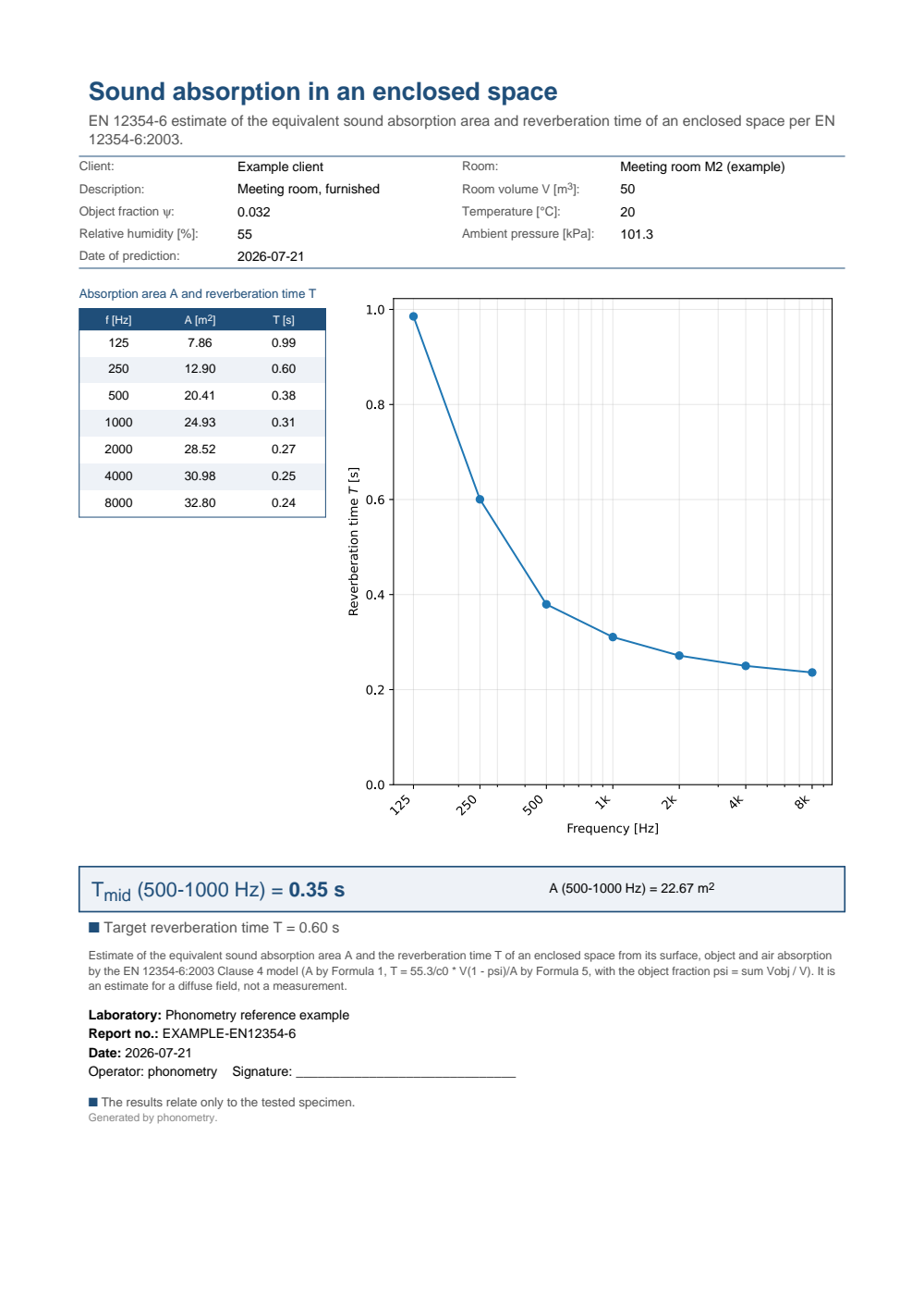
One-page EN 12354-6 enclosed-space fiche: a metadata header (client, room, description, room volume, object fraction, temperature, humidity and pressure), the octave-band table of the equivalent sound absorption area A and the reverberation time T from 125 Hz to 8 kHz beside the reverberation-time plot, and the boxed mid-frequency reverberation time with the mid-frequency absorption area alongside (no PASS/FAIL verdict).

Download the report (PDF)

Enclosed-space fiche (ReverberationResult.report), the per-band A/T table and the boxed T_mid.

What this guide covers

• Covered

  EN 12354-6:2003 Clause 4: the total equivalent sound absorption area of Formulae 1 to 4 with its surface, object, object-array and air terms (room.equivalent_absorption_area, room.hard_object_absorption, room.object_fraction, room.air_absorption_area), the Formula 5 reverberation time (room.reverberation_time), the per-octave-band chain (room.enclosed_space_reverberation) and the one-page fiche through .report(), validated against the three worked cases of Annex E. The input-data rules of clause 4.2, the interpretations of clause 4.5 and the limits of clause 4.6 are stated in §3, and the design inversion of Formula 5 in §2b.

• Not covered

  The informative Annex D method for irregular spaces and irregular absorption distribution, which is where the standard itself sends the cases that fail clause 4.6 (including its own Annex E case 3). The standard’s scope exclusions — very large or irregularly shaped spaces such as concert halls, theatres and factories — are outside the model rather than outside this implementation. Nothing here emits a verdict: EN 12354-6 gives a diffuse-field estimate, and a target passed through requirement is drawn as a reference line only.

See also

• Reverberation-time prediction (Sabine, Eyring, Arau): the classical family, and the models to reach for when the clause 4.6 limits fail.
• Room acoustic parameters (ISO 3382-1/2): the measured counterpart of the reverberation time predicted here.
• Sound Absorption Measurement and Rating: where the ${\alpha }_s$ come from (ISO 354) and where ${\alpha }_w$ is defined (ISO 11654) — the rating §3 forbids as an input.
• Predicting Sound Insulation (EN 12354): the family member that consumes the $A$ computed here, through $D_{nT}=D+10\lg (T/T_0)$ and $R^{\prime }=D+10\lg (S/A)$.
• Conformance report: the three Annex E cases these implementations are checked against.
• Outdoor Sound Propagation: the full ISO 9613-1 atmospheric-absorption model, for conditions or frequencies the six built-in climate profiles do not cover, via environment.propagation.air_absorption.
• API reference: room.enclosed_space_absorption.
• Theory: Sound insulation and absorption, predicted: the equivalent-absorption-area definition the EN 12354-6 procedure computes.

References

• European Committee for Standardization. (2003). Building acoustics — Estimation of acoustic performance of buildings from the performance of elements — Part 6: Sound absorption in enclosed spaces (EN 12354-6:2003). The Clause 4 model, its input-data rules and its validity limits: the total equivalent absorption area (clause 4.3, Formulae 1-4, Table 1) and the reverberation time (clause 4.4, Formula 5), validated against the three worked cases of Annex E. The linked catalogue record is the BSI Knowledge page for BS EN 12354-6:2003.
• International Organization for Standardization. (1993). Acoustics — Attenuation of sound during propagation outdoors — Part 1: Calculation of the absorption of sound by the atmosphere (ISO 9613-1:1993). Only the six climate-condition power attenuation coefficients of EN 12354-6 Table 1, derived from this standard for the 125 Hz-8 kHz octave bands; the full atmospheric-absorption model for arbitrary conditions and frequencies lives in the Outdoor Sound Propagation guide.
• International Organization for Standardization. (2003). Acoustics — Measurement of sound absorption in a reverberation room (ISO 354:2003). The laboratory measurement the surface and array coefficients come from.
• Kuttruff, H. (2016). Room acoustics (6th ed.). CRC Press. https://doi.org/10.1201/9781315372150The statistical reverberation theory the standard's formulae specialise.