Predicting Sound Insulation (EN 12354)
Standards: EN 12354Key references: Hopkins 2007
A laboratory rating describes an element in isolation; a building also transmits sound along every flanking path. This page covers the EN 12354 prediction of in-situ performance between rooms from laboratory element data: the airborne model of EN 12354-1 with its junction vibration reduction indices, the impact model of EN 12354-2 and the prediction fiches of both. The third and fourth parts of the same family, which cross the building envelope instead of an internal partition, are in Façade Sound Insulation. The measured quantities the model is checked against live in Field Insulation Measurement (ISO 16283); the laboratory inputs come from Laboratory Insulation Measurement.
How do I predict sound insulation with EN 12354 in Python?
Section titled “How do I predict sound insulation with EN 12354 in Python?”Build the three flanking paths of each junction with
building.flanking_element(), then combine them with
building.predicted_airborne_insulation(r_direct=57.0, flanking_paths=paths).
For the EN 12354-1 Annex H.3 example below it returns r_prime_w = 52.2 dB,
that is = 52 dB, and names the dominant path. Impact insulation goes
through predicted_impact_insulation().
Predicting performance (EN 12354)
Section titled “Predicting performance (EN 12354)”A laboratory rating describes an element in isolation, yet the sound a building actually transmits also travels around the partition (along the floor, up the façade, through the flanking walls), re-radiating into the receiving room. This flanking transmission is the whole difference between the laboratory and the field . EN 12354 predicts the in-situ apparent rating from the laboratory ratings of the elements plus the vibration transmission of their junctions.
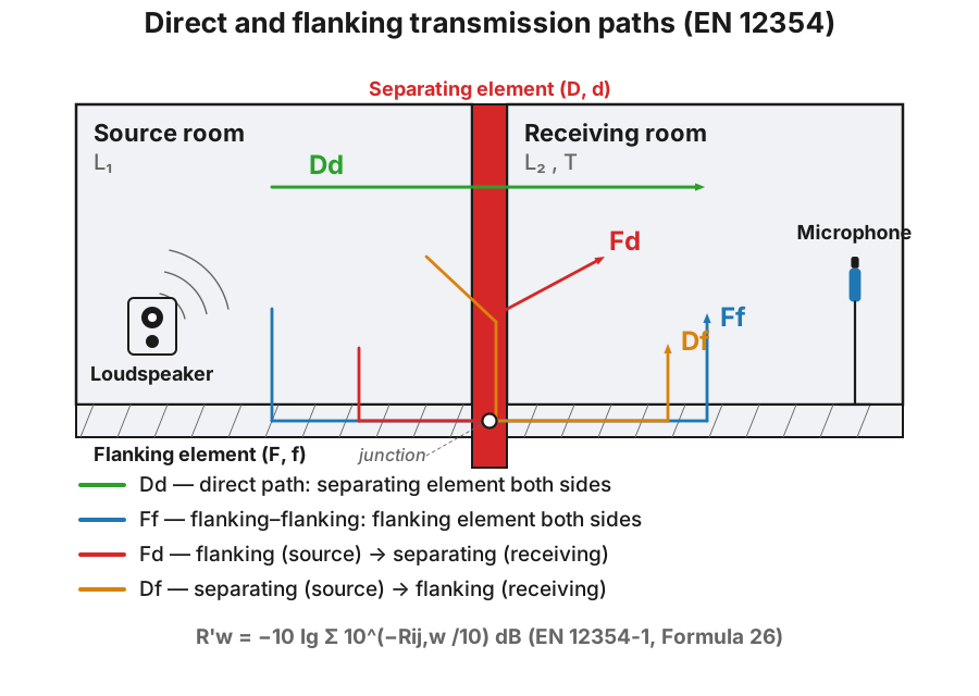
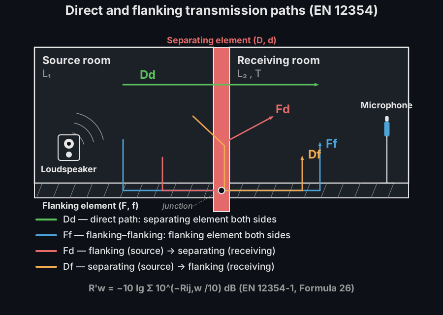
Each junction between a flanking element and the separating element carries three paths, (flanking→flanking), (direct→flanking) and (flanking→direct), alongside the single direct path .
Energy pulses leave the source room over the direct Dd path and the flanking Ff, Fd and Df paths, shrinking at each element and junction, and every path label lights up as its pulse re-radiates into the receiving room.
Energy pulses leave the source room over the direct Dd path and the flanking Ff, Fd and Df paths, shrinking at each element and junction, and every path label lights up as its pulse re-radiates into the receiving room.
The simplified single-number model combines them energetically (Formula 26):
with the direct path (Formula 27) and each flanking path (Formula 28a)
where m is the reference coupling length, the junction coupling length and the junction’s vibration reduction index.
Reading
Section titled “Reading Kij” is a property of the junction alone, and that is the whole point of it.
It is the average of the two velocity level differences measured across the
junction, corrected for the coupling length and for the equivalent absorption
lengths of the two elements, so the same junction carries the same
whatever building it is built into (which is what lets a catalogue of junction
types exist). Bigger is better: enters Formula (28a) with a plus sign, so
a high value is a junction that does not pass vibration on. The ranges are worth
carrying in your head. A rigid cross junction of similar masses sits around
8–13 dB and a rigid T junction about 3 dB lower (Annex E.3.2/E.3.3 give
and ); the
corner and thickness-change junctions of Annex E.3.6 fall to dB
(floored at dB) and dB, so at the worked example’s mass ratio
they return 0,1 dB and dB, a junction that hides nothing; and a
resilient interlayer or a lightweight double-leaf junction can exceed 20 dB
(the same mass ratio through a flexible_t gives 20,9 dB). That upper range is
what makes the internal wall of the worked example below almost invisible: it is
the weakest element on the list at = 33 dB, yet the 33,5 dB tabulated for
its takes its Ff path out of the sum entirely. On this model a bad
element behind a good junction beats a good element behind a bad one. For the
simplified model the Annex E values are read once, at 500 Hz, and stand in for a
quantity that is only approximately frequency-independent.
The mass argument is the place readers come unstuck. The Annex E fits are
quadratic in : the base-ten logarithm of the
mass ratio, with the element carrying the path and the
perpendicular element of the junction (Formula E.3). The library takes the
mass ratio itself and forms internally, so mass_ratio=1.61 means the
perpendicular element is 1,61 times as heavy per unit area. Any positive number
is accepted, so passing an already-logged value returns a plausible but wrong
answer: junction_vibration_reduction("rigid_cross", "through", 0.2068) returns
dB where the answer is 12,5 dB. And because is the element in
the transmission path, the same junction has a different mass ratio for
and for : the ratio is per path, not per junction.
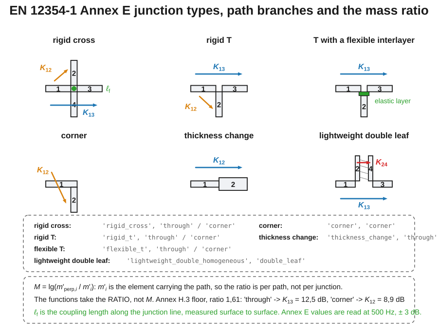
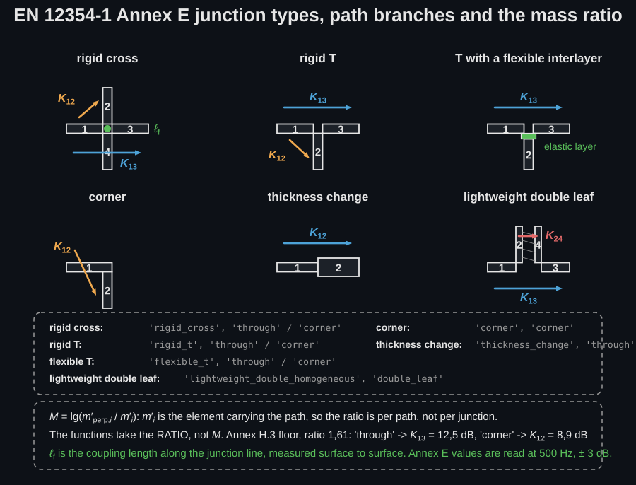
Each drawing above maps onto one (junction_type, path) argument pair, and the
path branch matters as much as the junction type: on the same rigid cross of the
worked example, path='through' gives 12,5 dB and path='corner' 8,9 dB.
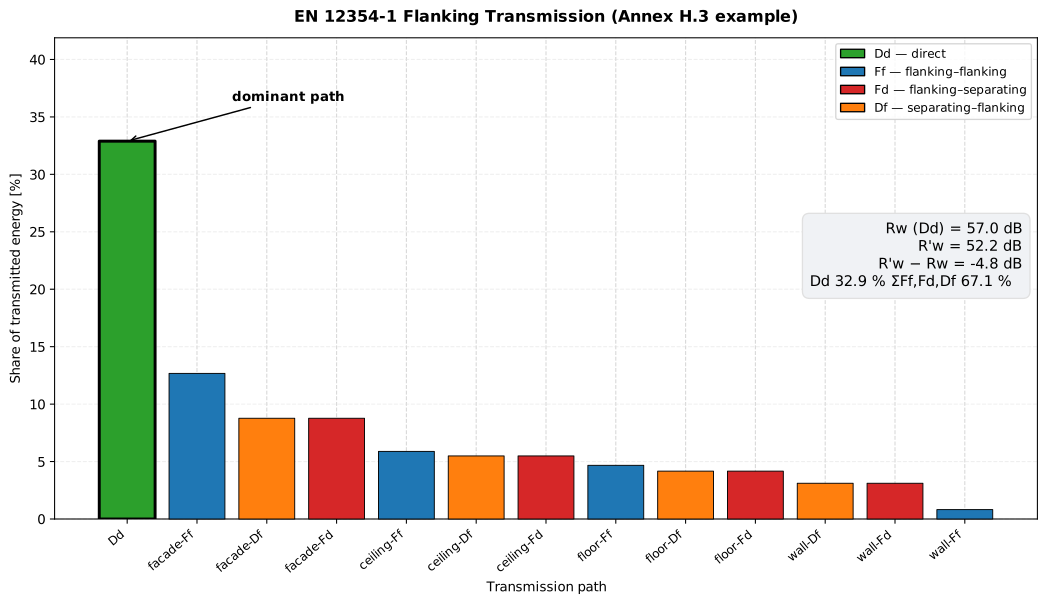
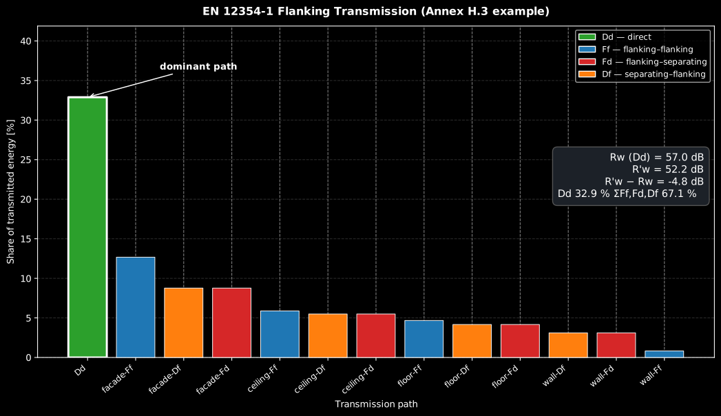
Per-path indices above, share of transmitted energy below. The direct path is the strongest single contributor at 33 %, yet two thirds of what arrives in the receiving room has gone around the wall, which is the 5 dB between dB and dB. The dashed line is the assembled , which necessarily sits below every individual path.
import numpy as npfrom phonometry import building
# EN 12354-1 Annex H.3: a separating wall Rs,w = 57 dB, area Ss = 11.5 m², with# four flanking elements. The simplified model reads each junction's Kij at# 500 Hz from the mass ratio m'perp / m' (Annex E) — here the floor's rigid# cross-junction (the mass ratio is itself rounded, hence 12.5 vs Annex 12.4):print(round(building.junction_vibration_reduction("rigid_cross", "through", 1.61), 1))  # 12.5  KFfprint(round(building.junction_vibration_reduction("rigid_cross", "corner",  1.61), 1))  #  8.9  KFd = KDf
# Build each element's three flanking paths (Ff, Df, Fd) from the Annex H# tabulated Kij, then combine the direct path Dd energetically (Formula 26).elements = [   # (name, Rw, KFf, KFd = KDf, coupling length lf)    ("floor",    49, 12.4,  8.9, 4.50),    ("ceiling",  46, 14.4,  9.2, 4.50),    ("facade",   42, 12.6,  6.7, 2.55),    ("int-wall", 33, 33.5, 15.7, 2.55),]paths = []for name, rw, k_ff, k_fd, lf in elements:    paths += building.flanking_element(label=name, r_flanking=rw, r_separating=57,                              k_ff=k_ff, k_fd=k_fd, k_df=k_fd,                              separating_area=11.5, coupling_length=lf)
res = building.predicted_airborne_insulation(r_direct=57.0, flanking_paths=paths)print(round(res.r_prime_w, 1))                          # 52.2  ->  R'w = 52 dBprint(res.dominant.label, round(res.dominant.fraction, 2))   # Dd 0.33 (direct dominates)
res.plot()   # per-path share of the transmitted energy, largest first (needs matplotlib)
Show the code for this figure
import matplotlib.pyplot as pltfrom phonometry import building
# Build each element's three flanking paths (Ff, Df, Fd) from the Annex H# tabulated Kij, then combine the direct path Dd energetically (Formula 26).elements = [   # (name, Rw, KFf, KFd = KDf, coupling length lf)    ("floor",    49, 12.4,  8.9, 4.50),    ("ceiling",  46, 14.4,  9.2, 4.50),    ("facade",   42, 12.6,  6.7, 2.55),    ("int-wall", 33, 33.5, 15.7, 2.55),]paths = []for name, rw, k_ff, k_fd, lf in elements:    paths += building.flanking_element(label=name, r_flanking=rw, r_separating=57,                              k_ff=k_ff, k_fd=k_fd, k_df=k_fd,                              separating_area=11.5, coupling_length=lf)res = building.predicted_airborne_insulation(r_direct=57.0, flanking_paths=paths)
# Per-path sound reduction index and each path's share of the transmitted# energy for the Annex H.3 result computed above.labels = [p.label for p in res.paths]r_w = [p.r_w for p in res.paths]frac = [100.0 * p.fraction for p in res.paths]
fig, (ax1, ax2) = plt.subplots(2, 1, figsize=(9, 6), sharex=True)ax1.bar(labels, r_w, color="tab:blue")ax1.axhline(res.r_prime_w, ls="--", color="k", label=f"R'w = {res.r_prime_w:.1f} dB")ax1.set_ylabel("Path Rij,w [dB]"); ax1.legend()ax2.bar(labels, frac, color="tab:orange")ax2.set_ylabel("Energy share [%]"); ax2.set_xlabel("Transmission path")for ax in (ax1, ax2):    ax.tick_params(axis="x", rotation=45)fig.suptitle("EN 12354-1 Annex H.3 — flanking transmission")fig.tight_layout()plt.show()
Every added flanking path strictly lowers below the direct ;
res.paths exposes each path’s share of the transmitted energy so the dominant
path is visible.
Read the split as a budget, because that is the practical yield of the whole model. The direct path is the largest single contributor here and it still carries only 33 % of the transmitted energy: two thirds of what arrives has gone around the wall. So perfecting the separating wall (making it infinitely good, not merely better) removes at most a third of the total, which is dB. Specifying a heavier partition on this construction would be wasted money; the floor, the ceiling and the façade carry the rest, and a junction detail or a lining on them is what moves the answer. The rule generalises: the best achievable improvement from fixing one path is dB, so a path below about 10 % of the total is worth at most 0,5 dB and is not worth touching, while a path at 50 % is worth 3 dB and one at 80 % is worth 7 dB. Rank the paths, spend on the top of the list, and stop when the next one is under a decibel.
flanking_element is a convenience that builds one junction’s
three paths at once; the single-path constructor behind it, flanking_path,
builds one Ff, Df or Fd path at a time (Formula 28a). Clause 4.4.2 also
enforces a floor from the junction geometry
(Formula 29). Pass the flanking-element area to
flanking_element(..., flanking_area=...) and the clamp is applied
automatically per path; or compute the floor yourself with
junction_min_vibration_reduction and pass it to
flanking_path(..., kij_min=...), which raises a below-floor to the
minimum.
Why a floor at all? is defined relative to the equivalent absorption lengths of the two elements, so on small elements the normalisation itself limits how much junction isolation may be claimed: energy arriving at a small, lightly damped element has nowhere to be dissipated except back across the junction it came through. The floor therefore rises as the elements shrink or the coupling length grows. On dwelling-scale elements it is normally negative and inactive; a prediction in which the clamp is active is a signal that an Annex E tabulated value is being applied outside the geometry it was fitted on.
from phonometry import building# Kij,min = 10 lg[lf·l0·(1/Si + 1/Sj)]; large elements give a low (here negative)# floor, so a realistic tabulated Kij is rarely clamped; but small, light# elements can push it above the tabulated value (e.g. lf = 4 m, S = 1.5 m²# gives 7.3 dB, over the 5 dB lightweight floor).print(round(building.junction_min_vibration_reduction(coupling_length=4.5, s_i=11.5, s_j=11.5), 1)) # -1.1Two linings on one path do not add
Section titled “Two linings on one path do not add”delta_r_ff, delta_r_fd, delta_r_df and flanking_path’s delta_r are each
the combined improvement of one whole path, not one lining’s rating. A path
usually has two ends, and both may be lined: a wall lining on the source side and
a suspended ceiling on the receiving side both sit on the same path. They do
not add. ISO 12354-1:2017 Formula (22) for the direct path and Formula (23) for
each flanking path both give
with the rule that decides which of the two: half the value is taken for the lining with the lower value; however, if both linings have a negative value, half the value is taken for the lining with the higher value. So two linings of +12 dB and +6 dB give 12 + 3 = 15 dB, not 18; and two of dB and dB give dB, because with both negative it is the less negative one that is halved. The sign rule inverts which lining is halved, and it is the part a careful reader still gets wrong.
The physics behind the halving is that two linings in series on the same
vibrational path are not independent: the second one operates on a field the
first has already reduced, so its full rating (measured on a bare element) is
not available a second time. ISO 12354-2 Clause 4.3.3 carries the same rule where
a floor covering and a receiving-side lining coexist. The direct path takes its
own combined through delta_r_direct.
The impact counterpart (EN 12354-2, Formula 21) is a direct subtraction: , with the bare-floor equivalent level (Annex B), the covering improvement (ISO 717-2) and the flanking correction from Table 1.
Check which edition your regulation cites. The model above is the EN 12354-2:2000 one, which condenses all flanking transmission into the single tabulated correction read from the separating and mean flanking masses. ISO 12354-2:2017 reorganised the same simplified model into explicit per-path formulae: (15) for the direct path and, for each flanking path, (16): the Table 1 correction is not in the current text at all, even though the underlying physics and the accuracy statement are unchanged. The 2017 edition also states a field of application the 2000 text left implicit (Clause 4.3.1): the simplified model is restricted to 100 Hz–3150 Hz, and for lightweight constructions to the measured normalised flanking impact level route of Formula (17). The frequency-band route of Detailed Sound Insulation Prediction is anchored on the 2017 editions throughout.
What the two mass inputs are, and where the closed form stops. Annex B’s
is not a theory: it is a regression fitted to measured
homogeneous heavyweight floors between 100 and 600 kg/m², and
equivalent_impact_level raises a UserWarning when it is called outside that
band. It works inside it because a bare massive slab’s impact level is set by its
mass and by the roughly constant loss factor of masonry construction. It fails
outside it because a light or ribbed floor radiates through its own resonances
rather than as a damped homogeneous plate, so the closed form is meaningless for
a hollow-core, beam-and-block or joisted deck at any mass, and an extrapolation
for a 900 kg/m² vault. The it wants is the mass of the bare structural
floor, without covering and without ceiling; the covering’s effect is
and is subtracted separately.
The flanking mass is a different quantity again: the arithmetic mean over the homogeneous flanking elements of the receiving room that carry no additional layer. A lined or dry-lined flanking wall is left out of the mean, not averaged in at its bare mass. Table 1 itself applies to the rooms-one-above-the-other case of the Annex E.3 example, and it is a discrete nearest-neighbour lookup, not an interpolation: 145 kg/m² and 150 kg/m² both return = 2 dB, and masses outside 100–900 kg/m² (separating) or 100–500 kg/m² (flanking) clamp to the nearest edge rather than extrapolating. Taken together, a lightweight building is outside this whole simplified impact route and needs the measured normalised flanking impact level path the 2017 edition prescribes.
from phonometry import building
# EN 12354-2 Annex E.3: a 0.14 m concrete floor (m' = 322 kg/m²) with a floating# floor (ΔLw = 33 dB), rooms one above the other, mean flanking mass 145 kg/m².ln_eq = building.equivalent_impact_level(322.0)                   # 164 - 35 lg(m')k = building.impact_flanking_correction(322.0, 145.0)             # Table 1 (sep 322, flk 145)imp = building.predicted_impact_insulation(ln_w_eq=ln_eq, delta_l_w=33.0, k_correction=k)print(round(ln_eq, 1), k, round(imp.l_prime_n_w, 1))     # 76.2 2 45.2  ->  L'n,w = 45 dB
# The lookup is discrete: the next tabulated flanking mass gives the same K.print(building.impact_flanking_correction(322.0, 150.0))          # 2, unchanged
# Exact Formula (3): L'nT,w = L'n,w - 10 lg(0.032 V). Annex E.3's own rounding# of the factor to 10 lg(V/30) sits 0.18 dB below; both give L'nT,w = 43 dB.print(round(building.standardized_impact_level(imp.l_prime_n_w, 50.0), 1))   # 43.2  L'nT,w
imp.plot()   # the Formula (21) terms as bars: Ln,w,eq - dLw + K -> L'n,w (needs matplotlib)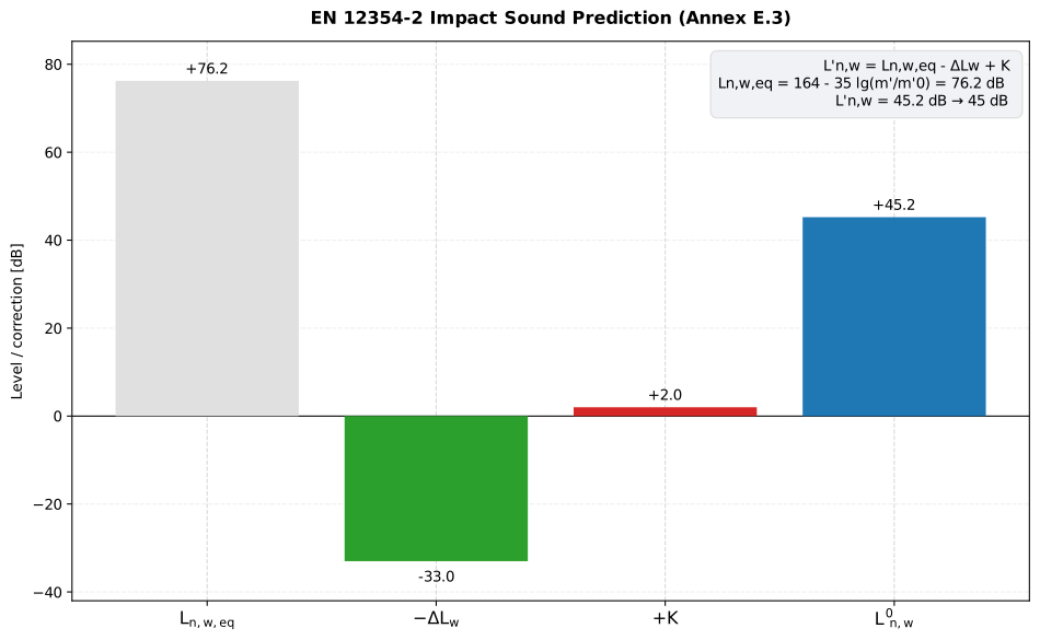
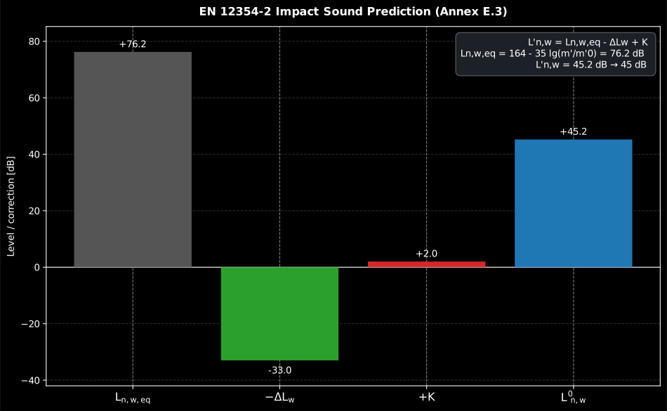
The whole EN 12354-2 simplified model is one subtraction: the massive bare floor starts at dB, the floating floor buys back 33 dB, and the flanking correction returns 2 dB, landing at dB.
Show the code for this figure
import matplotlib.pyplot as pltimport numpy as npfrom phonometry import building
# EN 12354-2 Annex E.3: 0.14 m concrete floor (m' = 322 kg/m2), floating# floor delta-Lw = 33 dB, mean flanking mass 145 kg/m2.ln_eq = building.equivalent_impact_level(322.0)k = building.impact_flanking_correction(322.0, 145.0)imp = building.predicted_impact_insulation(ln_w_eq=ln_eq, delta_l_w=33.0,                                           k_correction=k)
# One line — the Formula (21) terms as bars:imp.plot()plt.show()
# By hand, from the result's fields:labels = ["Ln,w,eq", "-dLw", "+K", "L'n,w"]values = [imp.ln_w_eq, -imp.delta_l_w, imp.k_correction, imp.l_prime_n_w]fig, ax = plt.subplots()ax.bar(np.arange(4), values)ax.axhline(0.0, color="k", lw=0.8)ax.set_xticks(np.arange(4), labels)ax.set_ylabel("Level / correction [dB]")ax.set_title(f"L'n,w = {imp.l_prime_n_w:.1f} dB (EN 12354-2 Annex E.3)")plt.show()
The airborne counterpart of that closure is Formula (5b),
, exposed as standardized_level_difference;
it closes the Annex H.3 example (standardized_level_difference(52.2, 50.0, 11.5) gives 53.6 dB, the printed chain 53.8 dB, both rounding to
dB).
The three insulation guides close a loop: the laboratory measures and element by element and junction by junction, this model assembles them into a predicted , and the field measurement checks the built result. When the measured value lands well below the prediction, look for a construction defect on the dominant path the model reports: a rigid bridge across a resilient junction, a missing lining, a leak around the separating element.
junction_vibration_reduction() / flanking_element() parameters
Section titled “junction_vibration_reduction() / flanking_element() parameters”| Parameter | Type | Units | Range / default | Notes |
|---|---|---|---|---|
junction_type | str | — | 'rigid_cross' / 'rigid_t' / 'flexible_t' / 'lightweight_facade' / 'lightweight_double_homogeneous' / 'lightweight_double_coupled' / 'corner' / 'thickness_change' | Junction geometry (Annex E.3-E.9) |
path | str | — | 'through' () / 'corner' () / 'double_leaf' () | Path branch |
mass_ratio | float | — | > 0 | (Formula E.2) |
frequency | float | Hz | default 500 | flexible_t and the E.7/E.8 double-leaf junctions are frequency-dependent |
r_flanking / r_separating | float | dB | — | Weighted indices of the flanking / separating element |
k_ff / k_fd / k_df | float | dB | — | Junction for the three paths |
separating_area | float | m² | > 0 | Separating-element area |
coupling_length | float | m | > 0 | Junction coupling length |
delta_r_ff / delta_r_fd / delta_r_df | float | dB | default 0 | Combined lining improvement of the whole path, both ends together (Formula 23) |
flanking_area | float | m² | default None | Flanking-element area ; enables the automatic clamp (Clause 4.4.2 / Formula 29) |
flanking_path() parameters
Section titled “flanking_path() parameters”| Parameter | Type | Units | Range / default | Notes |
|---|---|---|---|---|
label | str | — | — | Display name of the path |
kind | str | — | 'Ff' / 'Df' / 'Fd' | Which flanking branch the path is |
r_source / r_receive | float | dB | — | Weighted indices of the source-side / receive-side elements |
k_ij | float | dB | — | Junction vibration-reduction index for this path |
separating_area | float | m² | > 0 | Separating-element area |
coupling_length | float | m | > 0 | Junction coupling length |
delta_r | float | dB | default 0 | Combined lining improvement of this path, both ends together (Formula 23) |
kij_min | float | dB | default None | When given, k_ij is floored at this Formula (29) minimum |
predicted_airborne_insulation() returns an AirbornePredictionResult
(r_prime_w, r_direct_w, paths of PathContribution, dominant);
predicted_impact_insulation() an ImpactPredictionResult (l_prime_n_w,
ln_w_eq, delta_l_w, k_correction). The simplified model carries a reported
standard deviation of about 2 dB (Clause 5).
When the simplified model applies
Section titled “When the simplified model applies”Clause 4.4.4 of ISO 12354-1:2017 sets three conditions, and none of them is about arithmetic.
- Similar frequency dependence. The model assumes elements whose sound reduction index has a broadly similar shape against frequency, since it works on single numbers and a single number cannot carry two different shapes. A masonry wall flanked by masonry is the model’s home ground; a lightweight double-leaf partition beside a concrete floor is explicitly named as the case where the accuracy may be less.
- Dwelling-scale geometry. It applies mainly to dwellings whose element dimensions are similar to those of a test facility. Move far from that (a hall, a plant room, a very long junction) and the deviation grows.
- Adjacent rooms only. Clause 4.2.4 restricts the whole family to transmission between rooms that share the separating element, and secondary paths crossing more than one junction are neglected. Where the source is several junctions away, the EN 12354-5 route chains the junction indices instead.
And the ~2 dB standard deviation is not a tolerance on your answer. Clause 5 prints it assuming good workmanship and high measurement accuracy, and adds the advice that makes it usable: vary the input data, especially in complicated situations and with atypical elements, and read the spread in the result; Annex K systematises that into an uncertainty derived from the accuracy of every acoustic input.
The junction data deserve their own warning, because their spread is larger than the model’s. Annex E.3.1 states four things the page’s lookup does not show. Data exist only for junctions where the elements on either side in the same plane have the same mass. The measured points scatter by a typical ±3 dB about the printed lines, and “in some cases the deviation can be much larger due to variations in junction details and in workmanship”, which is larger than the ~2 dB of the whole model, so on most real predictions the junction input, not the summation, dominates the error. The values were deduced so that the estimated junction velocity level difference is right on average, which puts them generally 5 dB below the direction-averaged junction velocity level difference, so a measured cannot be substituted for a without that step. And the frequency independence holds “at least in the frequency range from 125 Hz to 2 000 Hz”; outside it the frequency effect can be larger. The way out is measured data: ISO 10848-4 for heavy junctions (which Annex E.3.1 itself recommends gathering at national level) and the flanking laboratory where the junction is lightweight, non-homogeneous or simply not in the catalogue.
EN 12354 prediction report (.report())
Section titled “EN 12354 prediction report (.report())”Both prediction results write a one-page prediction report through a
report(path) method. Unlike the measurement fiches, the reported result is an
estimate of the in-situ performance from the elements’ laboratory data plus
the flanking transmission across the junctions; the sheet states this
explicitly and is labelled a prediction, never a measurement.
AirbornePredictionResult.report() renders the predicted apparent sound
reduction index fiche (the transmission-path table beside the per-path
share-of-energy plot, the boxed ); ImpactPredictionResult.report()
renders the predicted apparent impact-level fiche (the Formula (21) term table
beside the term plot, the boxed ). Each names EN/ISO 12354-1/-2 and the
ISO 717 rating part in its basis line, prints the model’s ~2 dB standard
deviation and, when a requirement is supplied, adds a PASS/FAIL verdict
(airborne passes at or above it, impact at or below it).
verbose=True annexes each transmission path’s share of the transmitted energy
to the airborne table. Metadata, language="es" and the phonometry[report]
extra behave exactly as in the measurement fiches; the applicable
ReportMetadata fields are the separating element (specimen), the
separating-element or floor area (area), the room geometry (source_volume,
receiving_volume), the bare floor’s mass (mass_per_area, impact), the
manufacturer (manufacturer), the test room or facility (test_room), the
calculator/laboratory identity (client, laboratory, operator,
report_id, test_date) and a free-text summary of the flanking construction
and model assumptions (notes).
from phonometry import building, ReportMetadata
# Airborne prediction (EN 12354-1 Annex H.3): a separating wall Rs,w = 57 dB# flanked by four elements -> R'w = 52 dB.paths = []for label, rw, kff, kfd, lf in [    ("floor", 49.0, 12.4, 8.9, 4.5), ("ceiling", 46.0, 14.4, 9.2, 4.5),    ("facade", 42.0, 12.6, 6.7, 2.55), ("intwall", 33.0, 33.5, 15.7, 2.55),]:    ff, df, fd = building.flanking_element(        label=label, r_flanking=rw, r_separating=57.0,        k_ff=kff, k_fd=kfd, k_df=kfd, separating_area=11.5, coupling_length=lf)    paths += [ff, df, fd]air = building.predicted_airborne_insulation(r_direct=57.0, flanking_paths=paths)air.report("Rpw_prediction.pdf", metadata=ReportMetadata(    specimen="Separating wall, Rs,w = 57 dB", area=11.5,    source_volume=53.0, receiving_volume=50.0, requirement=50.0,    notes="Flanking: floor/ceiling/facade/internal wall."))   # R'w = 52 dBair.report("Rpw_prediction_paths.pdf", verbose=True)           # + energy share
# Impact prediction (EN 12354-2 Annex E.3): a concrete floor (m' = 322 kg/m²)# with a floating floor (ΔLw = 33 dB) -> L'n,w = 45 dB.ln_eq = building.equivalent_impact_level(322.0)k = building.impact_flanking_correction(322.0, 145.0)imp = building.predicted_impact_insulation(ln_w_eq=ln_eq, delta_l_w=33.0, k_correction=k)imp.report("Lnw_prediction.pdf",           metadata=ReportMetadata(mass_per_area=322.0, requirement=53.0))  # L'n,w = 45 dB
Both example fiches are regenerated with make reports and kept rendered in
the repository; click either preview to open the PDF.
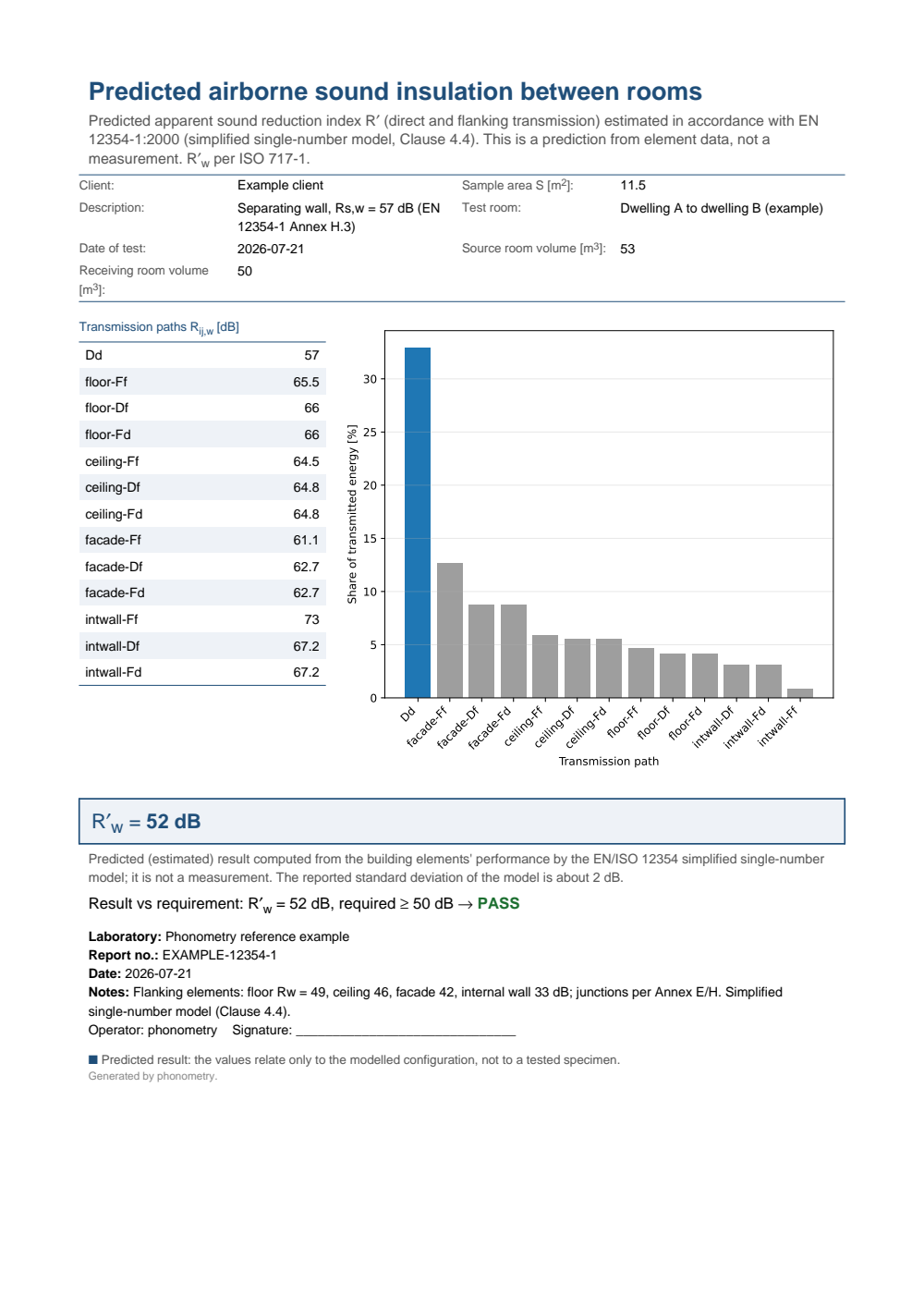
One-page predicted airborne sound insulation report between rooms (EN 12354-1 Annex H.3): the metadata header (separating element, area, room volumes), the transmission-path table (the direct path and each flanking path's weighted index Rij,w) beside the per-path share-of-energy bar chart, the boxed predicted R'w = 52 dB, the prediction statement noting the model's ~2 dB standard deviation and a PASS verdict against the 50 dB requirement.
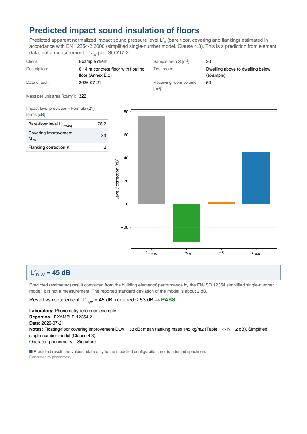
One-page predicted impact sound insulation report for a floor (EN 12354-2 Annex E.3): the metadata header, the Formula (21) term table (the bare-floor equivalent level Ln,w,eq, the covering improvement ΔLw and the flanking correction K) beside the term bar chart, the boxed predicted L'n,w = 45 dB, the prediction statement and a PASS verdict against the 53 dB requirement (a lower impact level is better).
Across the envelope: Parts 3 and 4
Section titled “Across the envelope: Parts 3 and 4”The two remaining parts of EN 12354 predict the same way but across the building envelope rather than between two rooms: EN 12354-3 the airborne insulation against outdoor sound, EN 12354-4 the sound power an indoor source radiates outwards. Both are built on the same area-weighted summation of element transmission factors used above, and both are covered, beside the ISO 16283-3 measurement they are compared against, in Façade Sound Insulation.
What this guide covers
Section titled “What this guide covers”Covered
The simplified single-number models of EN 12354-1:2000 (Clause 4.4) and EN 12354-2:2000 (Clause 4.3). Airborne: the Formula (26) energetic sum of the direct and flanking paths through
building.flanking_path,building.flanking_elementandbuilding.predicted_airborne_insulation, with the Annex E vibration reduction indices (rigid cross and T junctions, flexible interlayers, lightweight façades and double-leaf walls, corners and thickness changes) and the Clause 4.4.2 floor viabuilding.junction_vibration_reductionandbuilding.junction_min_vibration_reduction. Impact: the Formula (21) subtraction throughbuilding.equivalent_impact_level,building.impact_flanking_correction,building.predicted_impact_insulationandbuilding.standardized_impact_level. Both results write a prediction fiche with.report().Not covered
The detailed per-band models of both parts are the subject of Detailed Per-Band Prediction (ISO 12354): the same standard run band by band, with the laboratory element and junction data converted to their in-situ values before the paths are formed. Use the simplified model here when only the weighted element ratings are known and the question is whether the room passes; use the detailed one when the element spectra exist and the question is which path sets which band. The element inputs themselves (, , , mass per unit area) are taken as given, from laboratory data or from the mass-law estimates of Predicting Panel Sound Insulation. The rest of the family is covered by its own guides: EN 12354-3 and EN 12354-4 across the building envelope in Façade Sound Insulation, EN 12354-5’s service equipment in Installed structure-borne sound and EN 12354-6’s absorption model in Sound absorption in enclosed spaces.
References
Section titled “References”- European Committee for Standardization. (2000). Building acoustics — Estimation of acoustic performance of buildings from the performance of elements — Part 1: Airborne sound insulation between rooms (EN 12354-1:2000). The simplified airborne flanking-transmission prediction (Annex E junctions, worked example H.3). The linked catalogue record is the BSI Knowledge page for BS EN 12354-1:2000.
- European Committee for Standardization. (2000). Building acoustics — Estimation of acoustic performance of buildings from the performance of elements — Part 2: Impact sound insulation between rooms (EN 12354-2:2000). The simplified impact flanking-transmission prediction (worked example E.3). The linked catalogue record is the BSI Knowledge page for BS EN 12354-2:2000.
- Hopkins, C. (2007). Sound insulation. Butterworth-Heinemann. https://doi.org/10.4324/9780080550473The full treatment of flanking transmission and the EN 12354 prediction framework, from the vibration reduction index to its statistical basis. ISBN 978-0-7506-6526-1.