Installed structure-borne sound (EN 12354-5)

EN 12354-5:2009 predicts the sound pressure level in a receiving room caused by building service equipment (pumps, fans, lifts, water installations) that injects structure-borne sound into the building. It closes the structural-vibroacoustics chain: the source is described by its characteristic structure-borne sound power level $L_{Ws,c}$, derived from the EN 15657 reception-plate measurement through the Formula (15)/(17) conversion and a mobility correction (not the raw plate-injected level; see EN 15657); the source and receiver point mobilities set how much power is actually coupled into the structure, and the building transmission carries it to the receiving room. The Annex I mobility correction installed_power_from_reception_plate refers the characteristic reception-plate level $L_{Ws,n}$ to the actual receiver, $L_{Ws,\mathrm{inst}}=L_{Ws,n}+10{\log }_{10}(Y_{\infty ,i}/Y_{\infty ,\mathrm{rec}})$ with $Y_{\infty ,\mathrm{rec}}=5\cdot 10^{-6}\text{m/(N⋅s)}$; with the source mobility instead it yields $L_{Ws,c}$ (Annex I.3, Table I.8).

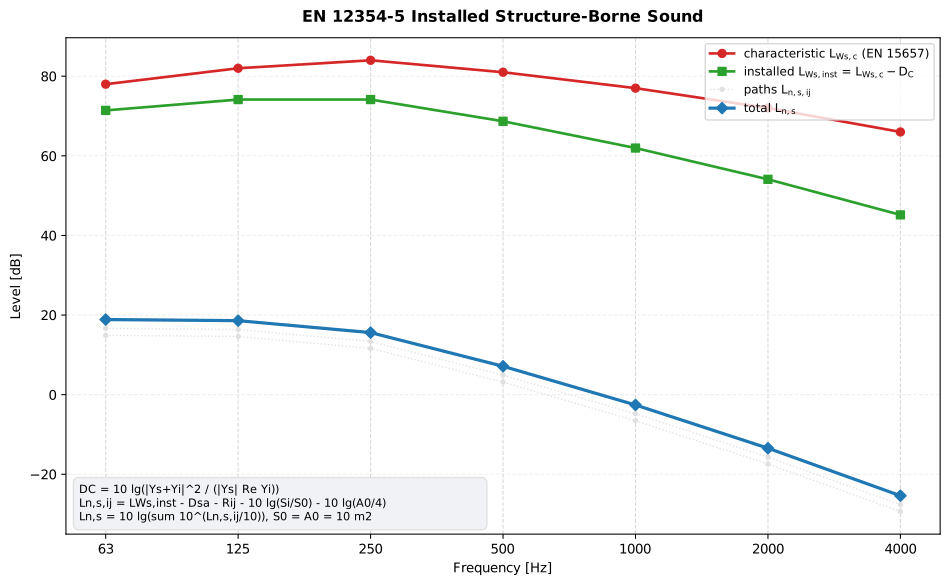
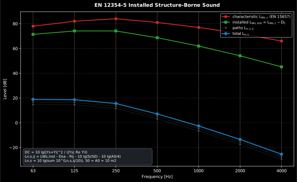
The whole chain on one axis, per octave band. The coupling term is not a fixed toll: it takes 6.6 dB out of the characteristic power at 63 Hz and 20.8 dB at 4 kHz, so the installed spectrum tilts down before any path is applied. Each path then subtracts its own $D_{sa}$, flanking index and area term, and here the smaller flanking wall beats the floor by 1.3 to 2.3 dB. The receiving-room level is the energetic sum of the paths, 2.0 to 2.4 dB above the stronger of the two: fixing only the worst path would buy about 2 dB, not the difference.

Show the code for this figure

import matplotlib.pyplot as plt
import numpy as np
from phonometry import building

# EN 15657 characteristic source power and illustrative point mobilities.
bands = np.array([63.0, 125.0, 250.0, 500.0, 1000.0, 2000.0, 4000.0])
lws_c = np.array([78.0, 82.0, 84.0, 81.0, 77.0, 72.0, 66.0])
ys = (2e-4 + 1e-4j) * (bands / 250.0)        # source mobility
yi = (3e-5 + 1e-5j) * np.ones_like(bands)    # receiver mobility
dc = np.array([float(building.coupling_term(a, b)) for a, b in zip(ys, yi)])

# Two transmission paths: the excited floor and a flanking wall. Dsa is
# negative and falls with frequency (Annex F.2), and enters with a minus sign.
paths = [
    {"adjustment_term": np.array([-14.0, -17.0, -20.0, -25.0, -30.0, -35.0, -40.0]),
     "element_area": 12.0,
     "flanking_reduction_index": np.linspace(44.0, 62.0, 7)},
    {"adjustment_term": np.array([-16.0, -19.0, -23.0, -28.0, -33.0, -38.0, -43.0]),
     "element_area": 9.0,
     "flanking_reduction_index": np.linspace(46.0, 64.0, 7)},
]
res = building.installed_source_prediction(lws_c, dc, paths, frequencies=bands)
res.plot()   # characteristic and installed power, per-path levels and the total
plt.show()

1. Coupling and installed power

Only part of the characteristic power is injected into the supporting element; the loss is the coupling term $D_C$, set for a point excitation by the source mobility $Y_s$ and the receiver mobility $Y_i$ (Formula 19b):

$$D_{C,i}=10{\log }_{10}\frac{|Y_s+Y_i{|}^2}{|Y_s|\mathrm{Re}\{Y_i\}},$$

which reduces to $10{\log }_{10}(|Y_s|/\mathrm{Re}\{Y_i\})$ for a force source (high source mobility, Formula 19c) and to $-10{\log }_{10}(|Y_s|\mathrm{Re}\{Z_i\})$ for a velocity source (low source mobility, Formula 19d); an elastic support adds its transfer mobility $Y_k$ inside the modulus (Formula 19e). The installed power level is then (Formula 18b) $L_{Ws,\mathrm{inst}}=L_{Ws,c}-D_C$.

The two limits are usable once the mobilities differ by about an order of magnitude: at $|Y_s|/|Y_i|=10$ the force-source form is 0.8 dB below the exact Formula 19b value and at 100 it is 0.1 dB below, while between those extremes the phase relationship decides the answer and Formula 19b must be evaluated with complex mobilities rather than magnitudes. Read the two idealisations physically: a force source imposes its force whatever the receiver does, so a stiffer receiver simply vibrates less and accepts less power, and $D_C$ stops depending on the receiver’s magnitude at all; a velocity source imposes its motion, so a stiffer receiver now takes more power out of it and the dependence inverts. A pump on a concrete slab is the textbook force source; a heavy machine bolted rigidly to a light timber floor is the case where the intuition flips, and the mid range — a mounted machine near its support resonance — is where $D_C$ is smallest and can even go negative, because the $|Y_s+Y_i{|}^2$ numerator collapses when the two mobilities are comparable and in antiphase. The exact curve bottoms out at matched mobilities, which is best power transfer and therefore worst isolation.

This is the same $L_{Ws,\mathrm{inst}}$ as the Annex I mobility correction of the introduction, reached by a different route: use Formula (18b) when $D_C$ is known from the two mobilities, and the direct correction $L_{Ws,n}+10{\log }_{10}(Y_{\infty ,i}/Y_{\infty ,\mathrm{rec}})$ when it is not. On the Annex I.3 cistern both give 68.2 dB at 63 Hz, from $L_{Ws,c}=84.4$ dB and $D_C=16.2$ dB. Note which quantity you are handed: $L_{Ws,c}$ is the input this page takes, and it is not the 68.2 dB the EN 15657 page prints as its installed level — feeding that in subtracts $D_C$ twice.

The physics behind $D_C$ is the classical power input of a point-excited plate: only the real part of the receiver’s driving-point mobility absorbs power, and the mismatch between $Y_s$ and $Y_i$ decides how much of the source’s capability ever enters the structure (Hopkins 2007, Section 2.8). The mobilities themselves come from the mechanical-mobility chain: measured per ISO 7626, or from the infinite-plate closed forms of panel theory when no measurement exists. A pump on a concrete slab is the textbook force source: its casing mobility is orders of magnitude above the slab’s, so $D_C$ collapses to Formula 19c and the injected power no longer depends on the receiver at all.

from phonometry import building

# A near-force source (Y_s >> Y_i) on a concrete floor:
dc = building.coupling_term(2e-4 + 1e-4j, 3e-5 + 1e-5j)
print(round(float(dc), 2))                                          # 9.86 dB
print(round(float(building.installed_structure_borne_power_level(82.0, dc)), 1))  # 72.1 dB

# The two limits, for comparison: |Y_s|/|Y_i| is only 7 here, so the
# force-source form is already 1.1 dB away from the exact Formula 19b value.
print(round(float(building.coupling_term_force_source(2e-4 + 1e-4j, 3e-5 + 1e-5j)), 2))      # 8.72
print(round(float(building.coupling_term_velocity_source(2e-4 + 1e-4j, 1 / (3e-5 + 1e-5j))), 2))  # -8.27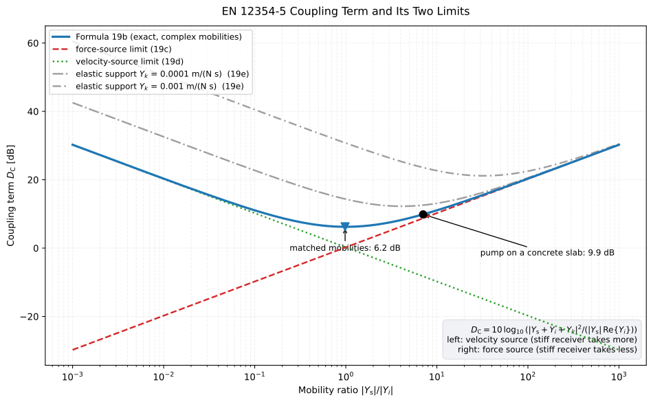

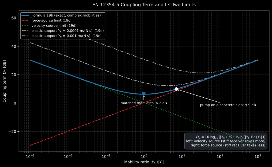
The whole of Formula 19b on one axis. Far to the right the source is a force source and $D_C$ follows $10\lg (|Y_s|/\mathrm{Re}\{Y_i\})$; far to the left it is a velocity source and follows $-10\lg (|Y_s|\mathrm{Re}\{Z_i\})$; the exact curve leaves both asymptotes within about a decade of matched mobilities, where it reaches its minimum of 6.2 dB — maximum power transfer, minimum isolation. The pump of the snippet sits at a ratio of only 7.1, which is why its exact 9.9 dB is 1.1 dB above the force-source limit. Adding an elastic support (Formula 19e) shifts the whole curve up: a transfer mobility of $10^{-4}$ m/(N·s) buys 2.7 dB at the pump’s ratio and one of $10^{-3}$ buys 13.7 dB, which is the isolation budget of a mount read straight off the coupling term.

Show the code for this figure

import matplotlib.pyplot as plt
import numpy as np
# `building` is the module imported by the snippet above.

yi = 3e-5 + 1e-5j                     # receiver mobility, fixed
ratio = np.logspace(-3.0, 3.0, 400)   # |Y_s| / |Y_i|
ys = abs(yi) * ratio * (2 + 1j) / abs(2 + 1j)

exact = np.array([float(building.coupling_term(a, yi)) for a in ys])
force = np.array([float(building.coupling_term_force_source(a, yi)) for a in ys])
velocity = np.array([float(building.coupling_term_velocity_source(a, 1 / yi))
                     for a in ys])

fig, ax = plt.subplots()
ax.semilogx(ratio, exact, label="Formula 19b (exact)")
ax.semilogx(ratio, force, "--", label="force source (19c)")
ax.semilogx(ratio, velocity, ":", label="velocity source (19d)")
for yk in (1e-4, 1e-3):               # elastic support, Formula 19e
    ax.semilogx(ratio, [float(building.coupling_term(a, yi, transfer_mobility=yk))
                        for a in ys], label=f"with $Y_k$ = {yk:g} m/(N·s)")
ax.plot(7.07, 9.86, "o")              # the pump of the snippet
ax.set(xlabel=r"Mobility ratio $|Y_\mathrm{s}| / |Y_i|$",
       ylabel=r"Coupling term $D_\mathrm{C}$ [dB]")
ax.legend()
plt.show()

Table D.1: $Y_s$ from the machine’s own parts

Nothing measures the source mobility of a boiler. Clause D.1.3 builds it instead out of the parts that carry the vibration to the feet, and Table D.1 gives the six closed forms it uses. typical_element_mobility is that table:

Row	Describing quantities	$|Y|$ in m/N.s
"mass"	$M$ [kg]	$[2\pi fM{]}^{-1}$
"bar_end"	$\rho$ [kg/m3], $c_L$ [m/s], $S$ [m²]	$[\rho c_{L}S{]}^{-1}$
"beam"	$\rho$, $c_L$, $t$ [m], $w$ [m]	$[7,6\rho tw\sqrt{c_{L}tf}{]}^{-1}$
"plate"	$\rho$, $c_L$, $t$ [m]	$[2,3c_L\rho t^2{]}^{-1}$
"pipe"	$\rho$, $c_L$, $t$ [m], $r$ [m]	$[63\rho tr\sqrt{c_{L}rf}{]}^{-1}$
"mass_spring"	$M$ [kg], $s$ [N/m], $\eta$ [-]	${\left[{\left(\frac{2\pi f\eta }{s(1+{\eta }^2)}\right)}^2+{\left(\frac{2\pi f}{s(1+{\eta }^2)}-\frac{1}{2\pi fM}\right)}^2\right]}^{1/2}$

Frequency is not in the “describing quantities” column, because it is the band frequency of the prediction rather than a property of the element — but it is in four of the six expressions, so those four rows take frequency and the other two refuse it. Pick the row by what actually carries the vibration: a small compact machine is its total mass, a machine on non-rigid feet is the mass-spring row, and the pipework leaving a pump is the pipe row. Note that "plate" is Formula (F.4) again, written in $\rho$, $c_L$ and $t$ instead of mass and bending stiffness — the same number as vibration.infinite_plate_mobility.

from phonometry import building

# A 120 kg pump on four rubber mounts, 1,0e6 N/m each, loss factor 0,1.
y_feet = building.typical_element_mobility(
    "mass_spring", frequency=125.0, mass=120.0, stiffness=4.0e6, loss_factor=0.1
)
print(f"{float(y_feet):.3g}")                       # 0.000185 m/(N.s)

# Well above the 29 Hz mount resonance the feet dominate: the casing on its
# own is an order of magnitude stiffer, so the mounts are what sets Y_s.
y_casing = building.typical_element_mobility("mass", frequency=125.0, mass=120.0)
print(f"{float(y_casing):.3g}")                     # 1.06e-05 m/(N.s)

dc = building.coupling_term(y_feet, 3e-5 + 1e-5j)   # onto a concrete floor
print(round(float(dc), 1))                          # 9.2 dB

The mass-spring row is the only one with a turning point. It is the series sum of a spring mobility and a mass mobility, so its second bracket holds the two reactances and they cancel at $f_0=(2\pi {)}^{-1}\sqrt{s(1+{\eta }^2)/M}$, leaving $|Y_s|$ at its damping-limited minimum — which is the frequency at which the mount injects the most power, because a small source mobility is a small $D_C$. That is the mounting resonance, and $\eta$ is the only thing setting how bad it gets. A row called with a quantity it does not describe, or with a frequency its expression does not contain, raises rather than quietly using a default.

Where the machine is fixed is part of $Y_i$

The receiver mobility is not a material constant of the element; it is a property of the point the machine is bolted to. EN 12354-5 Annex F.3 gives three routes to it, in decreasing order of authority.

Measured. Point mobilities at the actual contact points, normal to the surface, per ISO 7626-1 with single-point translational excitation per ISO 7626-2 (impact excitation per ISO 7626-5 is allowed), narrowband and then reduced to one-third octaves. The receiver must not be dynamically loaded while its mobility is measured — an important asymmetry with the source, which is isolated or freely suspended instead.

Calculated, mid-panel. For excitation in the centre area of a large homogeneous element, Formula (F.4) gives the real, frequency-independent infinite-plate value $Y_{i,\infty }=1/(8\sqrt{m^{\prime }{B}^{\prime }})=(2,3c_L\rho t^2{)}^{-1}$, which is vibration.infinite_plate_mobility(B, m) in the library. It is valid only above the element’s lowest resonance $f_{11}=(c_0^2/4f_c)(1/l_1^2+1/l_2^2)$ (Formula F.5); below $f_{11}$ the mobility turns complex and is set by the stiffness of the element’s supports, not by its own mass and bending stiffness. For the 5,00 m × 4,00 m, 220 mm concrete floor of the worked building $f_{11}$ is 39 Hz, comfortably below the range, but for a 1,20 m × 0,80 m concrete plinth of the same thickness it is 781 Hz, right in the middle of it — so on small stiff elements the closed form is the wrong tool. Elements with beams split again (Formula F.3.2): below $f_{11}$ use the effective bending stiffness $\sqrt{B_x^{\prime }{B}_y^{\prime }}$; above it, excitation between the beams uses the plate field and excitation on a beam uses the beam’s own mobility.

Corrected for the fixing position. Near a rigid edge the real part collapses as $\mathrm{Re}\{Y_i\}=\mathrm{Re}\{Y_{i,\infty }\}[1-J_0(2k_{B}a)]$ (Formula F.6a, with a corner form F.6b), $a$ being the distance to the edge. This makes the fixing distance a design variable rather than a detail: on that same concrete floor at 63 Hz, bolting the machine 0,20 m from a wall leaves 6,5 % of the mid-panel real mobility — 11,9 dB less injected power — and 0,50 m leaves 37 %, worth 4,3 dB. Move a pump towards a junction and it feeds the building less.

import numpy as np
from scipy.special import j0

rho, c_l, t = 2200.0, 3800.0, 0.220         # concrete, 220 mm
m, b = rho * t, c_l**2 * rho * t**3 / 12.0  # mass per area, bending stiffness
y_inf = 1.0 / (8.0 * np.sqrt(m * b))        # Formula (F.4), mid-panel
print(f"{y_inf:.3g}")                       # 1.07e-06 m/(N.s)

f_c = 343.0**2 / (1.8 * c_l * t)            # critical frequency
f_11 = 343.0**2 / (4 * f_c) * (1 / 5.0**2 + 1 / 4.0**2)
print(round(f_c, 1), round(f_11, 1))        # 78.2 Hz, 38.6 Hz -> F.4 valid here

f, a = 63.0, 0.20                           # 0.20 m from a rigid edge
k_b = np.sqrt(2 * np.pi * f) * (m / b) ** 0.25
print(round(float(1 - j0(2 * k_b * a)), 3))                    # 0.065
print(round(float(-10 * np.log10(1 - j0(2 * k_b * a))), 1))    # 11.9 dB less

The transfer mobility $Y_k$ of Formula (19e) is not a plate quantity at all: it is the dynamic transfer stiffness of the mount, measured on the ISO 10846 rig. The fixing position and the mount’s data sheet both belong in the report’s notes, because they are the two things that make a repeat prediction reproducible.

Table F.1: the tapping machine as a substitution source

When the equipment itself cannot be characterised, clause D.1.2.3 lets you measure the building’s transmission with a source whose force level is known and substitute the equipment into it afterwards (Formula D.6). The ISO tapping machine is the practical choice on low-mobility receiving structures, and Table F.1 is its octave-band force level:

Octave band [Hz]	31,5	63	125	250	500	1000	2000	4000
$L_F$ [dB]	139	142	145	148	151	154	156	156

Two conditions travel with the table. The closed form the standard prints beside it, $L_F=10{\log }_{10}(2,5f/10^{-12})$ in octave bands and $10{\log }_{10}(0,8f/10^{-12})$ in one-third-octave bands, holds only “up till about 1000 Hz”: it gives 157 dB and 160 dB at 2 kHz and 4 kHz where the table flattens at 156 dB, so read the table where the table exists and the closed form only for the one-third-octave bands it does not tabulate. And the levels are re $10^{-6}$ N despite the “re 1 pN” the caption prints; see the errata registry.

Clause D.1.3 then treats the machine as a force source with the mass-like mobility of its 0,5 kg hammers, which turns the table into the two inputs this page takes: $L_{Ws,c}=L_F-5-10{\log }_{10}f$ (Formula D.9a) and $D_{C,i}=-10{\log }_{10}(\omega M{Y}_i)+10{\log }_{10}[1+(\omega M{Y}_i{)}^2]$ (Formula D.9b, which is Formula 19b with $Y_s=1/\mathrm{j}\omega M$).

import numpy as np
from phonometry import building

bands = np.array(building.TABLE_F1_OCTAVE_BANDS)
lf = building.tapping_machine_force_level()            # Table F.1
lw_c = building.tapping_machine_characteristic_power_level(bands, lf)
print(np.round(lw_c, 1))   # [119. 119. 119. 119. 119. 119. 118. 115.]

# Onto the 220 mm concrete floor of the previous section (Y_i = 1,07e-6).
dc = building.tapping_machine_coupling_term(bands, 1.07e-6)
print(np.round(lw_c - dc, 1))   # [79.3 82.3 85.3 88.3 91.3 94.3 96.3 96.3]

In one-third-octave bands the characteristic power comes out flat at 114 dB re 1 pW, which is Formula (D.9a)‘s own ”$\approx 115$ dB” and the flat thick curve of the standard’s Figure D.3.

2. Transmission to the receiving room

EN 12354 parts 1 and 2 handle rooms excited through the air and by the standard tapping machine; part 5 covers the sources that shake the building directly: pumps, fans, lifts, whirlpool baths, cisterns and the pipework that ties them into walls and floors. Once the installed power is in the structure, several elements radiate into the receiving room: the excited element itself and every element the vibration reaches across the junctions. Each excited-element/radiating-element pair $i\to j$ is a transmission path with its own adjustment term and flanking index:

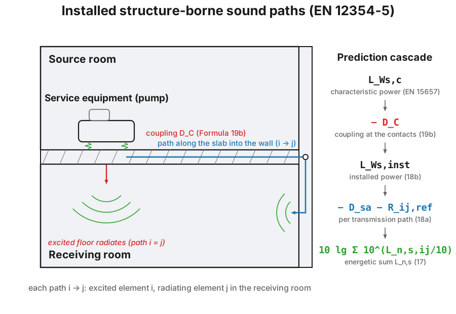
The diagram draws the simple case, one junction between the excited element and the radiator. In parts 1 and 2 the two rooms always share the separating element, and clause 4.2.4 of ISO 12354-1 says in so many words that the model describes transmission between adjacent rooms. Service equipment breaks that assumption routinely: the standard’s own flushing-cistern example puts the receiving room diagonally below the bathroom, and a riser or a lift shaft can be three junctions away from whoever complains. Annex F.1 says what to do. $K_{ij}$ then stops being the invariant of one junction and has to be read as covering the whole chain: the junction indices add along the path (Formula F.1), the intermediate elements’ equivalent absorption lengths may be taken numerically equal to their areas as a first estimate for large or well-damped elements, and an adjustment $\Delta K$ covers the longitudinal and in-plane waves that bending-wave theory misses — about 4 dB for two junctions and 6 dB for three or more, with the chained $K_{ij}$ floored near $-5$ dB, which corresponds to total structure-borne transmission. Two consequences for the input you supply here: an $R_{ij,\mathrm{ref}}$ computed for a single junction over-predicts the insulation of a multi-junction route, and several distinct routes usually join the same element pair, each of which must be counted as its own path or folded into one effective $R_{ij,\mathrm{ref}}$ first. Where the paths become many, Annex F.1 points at a full SEA model instead.

Each transmission path $i\to j$ gives a normalised sound pressure level from the installed power, the structure-to-airborne adjustment term $D_{sa}$, the flanking sound reduction index $R_{ij,\mathrm{ref}}$ (EN 12354-1) and the element area (Formula 18a):

$$L_{n,s,ij}=L_{Ws,\mathrm{inst},i}-D_{sa,i}-R_{ij,\mathrm{ref}}-10{\log }_{10}\frac{S_i}{S_0}-10{\log }_{10}\frac{A_0}{4},$$

with $S_0=A_0=10{\text{m}}^2$. Read the five terms in order, because each one undoes a different normalisation. $L_{Ws,\mathrm{inst},i}$ is the power that actually entered element $i$. $D_{sa,i}$ converts that structural excitation into the equivalent airborne excitation, so that the next term may be an airborne quantity at all. $R_{ij,\mathrm{ref}}$ is that airborne flanking index, defined for a reference element of $S_0=10{\text{m}}^2$. $10\lg (S_i/S_0)$ therefore puts the real element back: the same injected power spread over a larger element gives a smaller vibration amplitude per unit area, so a bigger $S_i$ lowers the radiated level. And $10\lg (A_0/4)$ turns radiated power into a reverberant sound pressure level, through the diffuse-field relation $p^2=4{\rho }_0{c}_{0}W/A$ evaluated at the reference absorption area $A_0$. That last term is what “normalised” means on this page: the result is the level the room would have if its equivalent absorption area were 10 m². A real room with more absorption than that measures lower; ISO 16032 field measurements of service equipment are usually standardised instead, referred to a reverberation time of 0,5 s, and the two are not interchangeable.

The paths then combine energetically, band by band (Formula 17):

$$L_{n,s}=10{\log }_{10}\sum _{ij}10^{L_{n,s,ij}/10}.$$

res.total_level is that per-band combination and res.overall_level the sum over the spectrum of it. For the flushing cistern of Annex I.3 the four paths total 41,4 dB at 63 Hz and the whole spectrum closes at 29 dB(A) — see the weighting note below the snippet.

The adjustment term $D_{sa}$

A point force pumps energy into free bending waves, while an incident sound field drives forced waves as well. $D_{sa}$ is the bookkeeping factor that lets the airborne flanking index $R_{ij,\mathrm{ref}}$ — an airborne quantity — be reused for a structurally excited element: it converts the injected structure-borne power into the incident airborne power that would leave the element with the same free-vibration energy (Formula 20a). For perpendicular force excitation of a homogeneous element that becomes Formula (20b),

$$D_{sa,i}=10{\log }_{10}\frac{2\pi m_{i}2.2{\tau }_i}{{\rho }_0{c}_0{T}_{s,i}{\sigma }_i}\text{dB},$$

with $R_i=-10{\log }_{10}{\tau }_i$, and Annex F.2 gives the working form

$$D_{sa,i}=10{\log }_{10}\frac{400f_{c,i}{\sigma }_i}{m_i{f}^2}\text{dB}\text{(Formula F.3)},$$

exact above the critical frequency (${\sigma }_i\approx 1$) and a good approximation over the whole range. Read it: heavier elements and higher frequencies make $D_{sa}$ more negative, at $-20{\log }_{10}f$ once $\sigma$ has saturated.

Caution

$D_{sa}$ is normally negative — pass the tabulated value with its printed sign. The standard’s own Annex I columns run from about $-14$ dB at 63 Hz to $-45$ dB at 2 kHz for ordinary concrete and masonry elements. The term enters Formula (18a) with a minus sign, so a negative $D_{sa}$ raises the predicted level. Earlier revisions of this page passed "adjustment_term": 5.0 and 6.0; copying that pattern with a real Annex F value in its place would leave the prediction roughly 20 to 40 dB low across the spectrum, with no error raised.

Every input of Formula (F.3) is already available: in_situ_element returns the in-situ structural reverberation time, the radiation factor and $R$ for the element, and structure_to_airborne_adjustment is Formula (F.3) itself.

import numpy as np
from phonometry import building

# Formula (F.3) for the 92 kg/m2 wall of the Annex I worked building.
f = np.array([63.0, 125.0, 250.0, 500.0, 1000.0, 2000.0])
sigma = np.minimum(1.0, np.sqrt(f / 200.0))        # radiation factor, fc = 200 Hz
dsa_f3 = building.structure_to_airborne_adjustment(
    f, critical_frequency=200.0, mass_per_area=92.0, radiation_factor=sigma
)
print(np.round(dsa_f3, 1))    # [-9.1 -13.6 -18.6 -24.6 -30.6 -36.6]  all negative

bands = np.array([250.0, 500.0, 1000.0])
res = building.installed_source_prediction(
    characteristic_power_level=np.array([80.0, 82.0, 78.0]),
    coupling_term=np.array([9.0, 10.0, 11.0]),
    paths=[
        {"adjustment_term": np.array([-19.0, -25.0, -31.0]),
         "flanking_reduction_index": np.array([50.0, 52.0, 55.0]), "element_area": 12.0},
        {"adjustment_term": np.array([-22.0, -28.0, -34.0]),
         "flanking_reduction_index": np.array([52.0, 54.0, 57.0]), "element_area": 8.0},
    ],
    frequencies=bands,
)
print(np.round(res.total_level, 1))      # total L_n,s per band
print(round(res.overall_level, 1))       # band-summed level [dB]

res.plot()   # the per-path and total L_n,s cascade, as in the figure above (needs matplotlib)

The InstalledSourceResult carries the per-path levels, the total per band, the installed power level and .overall_level, and its .plot() draws the whole cascade.

overall_level is not the number a regulation limits

overall_level is the plain energetic sum of the per-band $L_{n,s}$ over the bands you supplied. It is not A-weighted, and the quantity every national requirement for service-equipment noise is written in — and the quantity the ISO 16032 field measurement produces — is the A-weighted single number $L_{n,s}(A)$. Both of EN 12354-5’s worked examples close on one: 26 dB(A) for the Annex I.2 whirlpool bath and 29 dB(A) for the Annex I.3 cistern. The gap is not small. Service-equipment spectra are weighted to the low bands, exactly where the A-weighting is steepest, so for the Annex I.3 cistern the unweighted sum is 44,0 dB against the standard’s 29 dB(A) — fifteen decibels of headroom that does not exist. Weight the band levels before summing them:

import numpy as np

# Annex I.3 total per octave band, and the A-weighting corrections for those
# nominal centres (ISO 3744 Annex E Table E.2 / IEC 61672-1).
l_ns = np.array([41.4, 39.6, 30.5, 28.9, 18.5, 4.4])       # 63 Hz to 2 kHz
a_corr = np.array([-26.2, -16.1, -8.6, -3.2, 0.0, 1.2])
print(round(float(10 * np.log10(np.sum(10 ** (0.1 * l_ns)))), 1))            # 44.0 dB
print(round(float(10 * np.log10(np.sum(10 ** (0.1 * (l_ns + a_corr))))), 1))  # 29.3 dB(A)

Read a result against that scale, not against the unweighted total: 29 dB(A) for a cistern and 26 dB(A) for a whirlpool bath are what the standard’s own conforming examples produce, and dwelling limits for service equipment usually sit in the low thirties.

3. The prediction report (.report())

A prediction ends as a document. The InstalledSourceResult exposes a .report() method that writes a one-page PDF fiche, clearly labelled a prediction, not a measurement: a prediction-basis line naming EN 12354-5:2009, an optional metadata header (client, source equipment, receiving room, instrumentation, climate, date), a per-band table (nominal octave/one-third-octave frequency, the installed structure-borne power level $L_{Ws,inst}$, each transmission path’s normalised SPL $L_{n,s,ij}$ and the combined total $L_{n,s}$), the per-path and total $L_{n,s}(f)$ spectra, and a boxed band-summed total $L_{n,s}$ (dB) with the installed power total and the path count.

The metadata is supplied through a ReportMetadata, whose applicable fields here are the source equipment (specimen), the receiving room (test_room), the client, the instrumentation and the footer identity (laboratory, operator, report_id, notes). Supplying requirement adds a PASS/FAIL verdict against a declared upper limit on the overall $L_{n,s}$ (less is better). verbose=True adds one column per transmission path (up to five); otherwise only the installed power and the combined total are shown. language="es" renders the Spanish fiche with comma decimals. The basis strip states Formulae 18a/17 and the prediction disclaimer.

Two numbers in the snippet below are the standard’s, not invented: 16.2 is the coupling term of the Annex I.3 cistern at its wall contact, and the lwc array is that cistern’s characteristic power level, the 84,4 dB the EN 15657 page derives at 63 Hz. requirement is compared against overall_level, so the 45 dB below is an unweighted band-sum limit; a regulation stated in dB(A) has to be checked against the A-weighted sum of the previous section instead, and against this example’s spectrum the two differ by about 15 dB.

import numpy as np
from phonometry import ReportMetadata, installed_source_prediction

bands = np.array([63, 125, 250, 500, 1000, 2000], float)
lwc = np.array([84.4, 82.5, 69.9, 67.6, 61.6, 49.9])   # characteristic power [dB]
dsa = np.array([-13.6, -17.3, -17.4, -20.0, -26.9, -32.9])
paths = [
    {"adjustment_term": dsa,
     "flanking_reduction_index": np.array([43.0, 46, 50.2, 54.7, 64.6, 73]),
     "element_area": 12.8},
    {"adjustment_term": dsa,
     "flanking_reduction_index": np.array([37.0, 41.2, 35.9, 37.7, 49, 57.8]),
     "element_area": 12.8},
]
res = installed_source_prediction(lwc, 16.2, paths, frequencies=bands)

res.report(
    "installed_structure_borne.pdf",
    metadata=ReportMetadata(
        client="Example dwelling refurbishment",
        specimen="WC flushing cistern (wall-fixed)",
        test_room="Receiving room: adjacent bedroom",
        report_id="EXAMPLE-12354-5",
        requirement=45.0,
    ),
)   # overall L_n,s ~ 43 dB -> declared limit 45 dB: PASS

The example fiche is regenerated with make reports and kept rendered in the repository; click the preview to open the PDF.

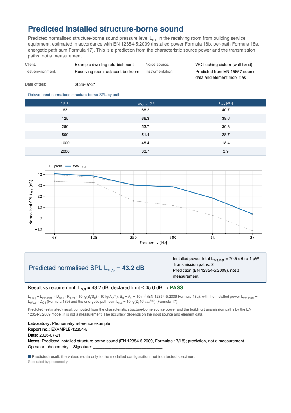
One-page EN 12354-5:2009 installed structure-borne sound prediction fiche, clearly labelled a prediction and not a measurement: a header with the client, the source equipment, the receiving room and the identity, the octave-band table (63 Hz to 2 kHz) of the installed structure-borne power level L_Ws,inst, the two flanking paths' normalised SPL L_n,s,ij and the combined total L_n,s, the per-path and total L_n,s(f) spectra, and the boxed band-summed total L_n,s with the installed power total and the path count, closed by a basis strip stating Formulae 18a/17 and the prediction disclaimer, with a PASS verdict against the declared 45 dB limit.

Download the report (PDF)

Installed structure-borne prediction fiche (InstalledSourceResult.report), an EN 12354-5 estimate of the normalised structure-borne SPL in the receiving room.

What this guide covers

• Covered

  EN 12354-5:2009: the coupling term $D_C$ (clause 4.4.3, Formulae 19b-e, with its force-source and velocity-source limits) via coupling_term, the installed power level $L_{Ws,\mathrm{inst}}=L_{Ws,c}-D_C$ (Formula 18b) via installed_structure_borne_power_level, and the per-path normalised sound pressure level and its energetic total (Formulae 18a, 17) via installed_source_prediction. Validated against the standard’s own Annex I worked examples, the whirlpool bath (I.2) and the flushing cistern (I.3), within the ±0.15 dB rounding of the printed intermediates. The informative tables of the annexes are here too: Table D.1 (mobility of typical construction elements) via typical_element_mobility, Table F.1 (force level of the ISO tapping machine) via tapping_machine_force_level with Formulae (D.9a) and (D.9b), the adjustment term of Formula (F.3) via structure_to_airborne_adjustment, and the multi-junction $\Delta K$ of clause F.1 via multi_junction_adjustment.

• Not covered

  The flanking reduction index $R_{ij,\mathrm{ref}}$ is an input you supply from measurement or from EN 12354-1; Annex F.1 gives only the multi-junction correction to it, not the index itself. Formula (F.1) for the equivalent $K_{ij}$ over several junctions, the SEA route of Formula (F.2) and the mobility corrections for excitation near a border or corner (Formulae F.6a and F.6b) are not implemented. Only the 2009 edition is implemented, not the 2023 revision.

See also

• Structure-borne sound power of equipment (EN 15657): the reception-plate characterisation that supplies $L_{Ws,c}$ and the source mobility this prediction consumes.
• Mechanical mobility and the FRF family (ISO 7626-1): the measured $Y_s$ and $Y_i$ behind the coupling term.
• Bending-wave transmission at plate junctions: the junction physics that carries the installed power to the flanking radiators.
• Predicting Sound Insulation (EN 12354): the airborne and impact members of the same prediction family.
• API reference: building.prediction.installed_structure_borne.
• Theory: Point mobilities and radiation efficiency: the mobility and radiation-efficiency theory the installed level is predicted from.

References

• Cremer, L., Heckl, M., & Petersson, B. A. T. (2005). Structure-borne sound: Structural vibrations and sound radiation at audio frequencies (3rd ed.). Springer. https://doi.org/10.1007/b137728The source-receiver mobility coupling and the structure-borne transmission across junctions behind the coupling term and the path model. ISBN 978-3-540-22696-3.
• European Committee for Standardization. (2009). Building acoustics — Estimation of acoustic performance of buildings from the performance of elements — Part 5: Sound levels due to service equipment (EN 12354-5:2009). The coupling term (clause 4.4.3, Formulae 19a-19e), the installed structure-borne power level (Formula 18b), the structure-to-airborne adjustment term (clause 4.4.4, Formulae 20a/20b), and the normalised sound pressure level per path and its energetic combination (Formulae 18a, 17). Conformance is anchored on the coupling-term force-source limit and the standard's own Annex I worked examples: the whirlpool bath of I.2 (Table I.6a: mobility correction and path 11) and the flushing cistern of I.3 (Tables I.8/I.9: source conversion, all four transmission paths, the Formula 17 total and its 29 dB(A) closure), within the ±0.15 dB rounding of the printed one-decimal intermediates. D_sa and R_ij,ref are inputs (from measurement / EN 12354-1 / Annexes D and F). The linked catalogue record is the BSI Knowledge page for BS EN 12354-5:2009; since revised as EN 12354-5:2023 (https://knowledge.bsigroup.com/products/building-acoustics-estimation-of-acoustic-performance-of-buildings-from-the-performance-of-elements-sounds-levels-due-to-the-service-equipment).
• Hopkins, C. (2007). Sound insulation. Butterworth-Heinemann. https://doi.org/10.4324/9780080550473Section 2.8 (driving-point impedance and mobility): the power a mechanical source injects into a plate through the source and receiver mobilities, the building-acoustics reading of the clause 4.4.3 coupling term. ISBN 978-0-7506-6526-1.