Mechanical mobility and the FRF family (ISO 7626-1)

Mechanical mobility is the complex ratio of a velocity response to the force that produces it, $Y=v/F$. It is one member of a family of motion-per-force frequency-response functions (FRFs): which one is used depends only on whether the motion is a displacement, a velocity or an acceleration, and each has a force-per-motion reciprocal. ISO 7626-1:2011 defines the whole family (Table 1, with the 3.1.2 mobility definition), and the classic closed-form single-degree-of-freedom (SDOF) resonator serves as the reference for those definitions. ISO 7626-2:2015 adds the measurement side: FRF estimation from measured signals and its acceptance criteria. This FRF backbone underpins the structure-borne source and transmission standards: ISO 9611, ISO 10846, EN 15657 and EN 12354-5.

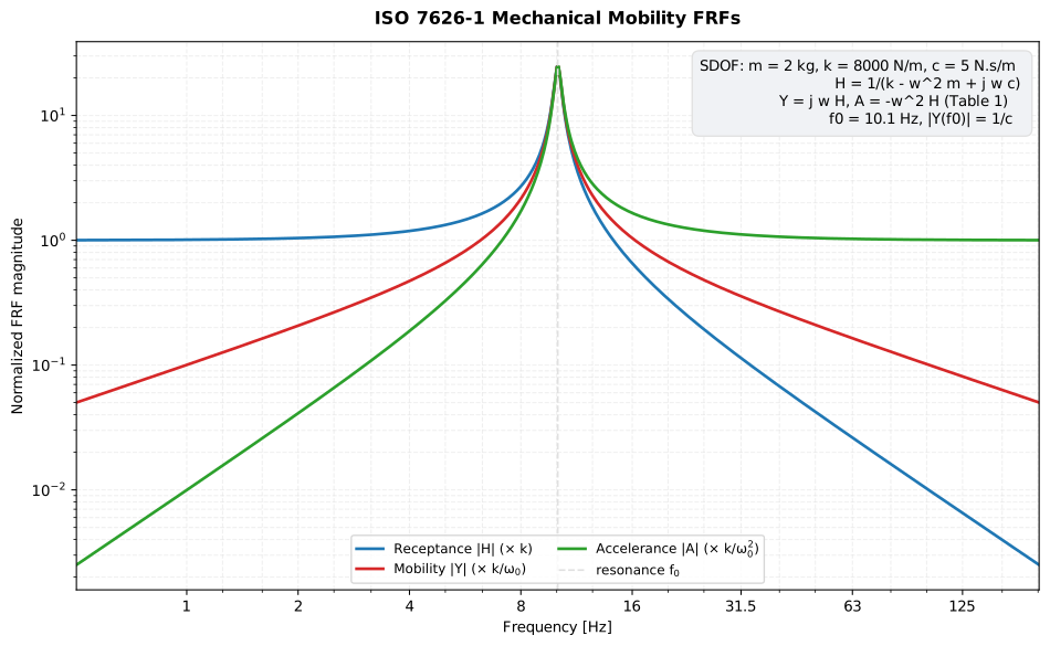
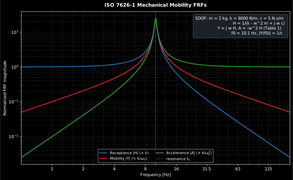
The whole Table 1 family in one picture. The three curves peak at the same frequency because they describe the same resonator; what distinguishes them is the slope on either side of it, which differs by one power of $\omega$ from one row of the table to the next. That is why receptance emphasises the low-frequency, stiffness-controlled end, accelerance the high-frequency, mass-controlled end, and mobility sits between them — and it is why mobility is the currency of power flow (section 1). Each curve is scaled by the constant printed in its legend entry — $k$, $k/{\omega }_0$ and $k/{\omega }_0^2$ — so the three peak at the same height and their shapes are comparable; the absolute levels differ by orders of magnitude.

Show the code for this figure

import matplotlib.pyplot as plt
import numpy as np
from phonometry import vibration

m, k, c = 2.0, 8000.0, 5.0
f0 = vibration.resonance_frequency(m, k)
f = np.logspace(np.log10(f0 / 20.0), np.log10(f0 * 20.0), 600)
w0 = 2.0 * np.pi * f0
h = vibration.sdof_receptance(f, m, k, c)
y = vibration.convert_frf(h, f, "receptance", "mobility")
a = vibration.convert_frf(h, f, "receptance", "accelerance")

# Scaled by a constant each, not normalised by their own maxima: the point
# is that the three differ in slope, and dividing by the peak hides it.
for label, frf in (("receptance |H| x k", np.abs(h) * k),
                   ("mobility |Y| x k/w0", np.abs(y) * k / w0),
                   ("accelerance |A| x k/w0^2", np.abs(a) * k / w0**2)):
    plt.loglog(f, frf, label=label)
plt.axvline(f0, ls="--", color="0.6")
plt.xlabel("Frequency [Hz]"); plt.ylabel("Scaled FRF magnitude")
plt.legend(); plt.show()

1. The frequency-response-function family (Table 1)

For a harmonic motion $x{e}^{j\omega t}$ the velocity is $j\omega x$ and the acceleration $-{\omega }^{2}x$, so all three motion-per-force FRFs follow from the receptance $H$ by a power of $j\omega$, and each has a force-per-motion reciprocal:

Motion	FRF (motion / force)	Unit	Reciprocal (force / motion)	Unit
displacement	receptance $H=x/F$	m/N	dynamic stiffness $1/H$	N/m
velocity	mobility $Y=j\omega H$	m/(N·s)	impedance $1/Y$	N·s/m
acceleration	accelerance $A=-{\omega }^{2}H$	1/kg	apparent mass $1/A$	kg

The figure at the top of this page is that table drawn: the same resonator seen through all three rows, differing by one power of $\omega$ each.

convert_frf moves between any two of the six FRFs, pivoting through the receptance. A driving-point FRF has the response and force at the same point ($i=j$); a transfer FRF has them at different points. Note that the force-per-motion kinds are element-wise reciprocals: the free quantities of ISO 7626-1, 3.1.4; the blocked matrix quantities of Table 1 do not invert element-wise for multi-coordinate systems (Table 1 also names $F/a$ the “effective mass”, the quantity called apparent mass here).

from phonometry import vibration

# A mobility of 2e-3 m/(N.s) at 80 Hz, expressed as the other FRFs:
Y = 2e-3
print(round(abs(vibration.convert_frf(Y, 80.0, "mobility", "impedance")), 1))     # 500.0  N.s/m
print(f"{abs(vibration.convert_frf(Y, 80.0, 'mobility', 'accelerance')):.3f}")    # 1.005  1/kg

The choice between the three motion FRFs is one of convenience, not physics: they carry the same information and convert_frf moves between them exactly. Accelerance is what an accelerometer-based measurement delivers directly; mobility is the natural currency of the structure-borne power standards (power is force times velocity, so $P=\frac{1}{2}\mathrm{Re}\{Y\}|F{|}^2$ at a contact); the reciprocals appear whenever a source is described by what it imposes rather than by how it responds. A driving-point mobility is read as three regimes — a stiffness line, a peak and a mass line — which section 4 shows on the plot.

Why two mobilities decide the power

That $P=\frac{1}{2}\mathrm{Re}\{Y\}|F{|}^2$ is only half the story, because the force at a contact is not given: it is what the two structures agree on. Couple a source of free velocity $v_f$ and mobility $Y_{\text{source}}$ to a receiver of mobility $Y_{\text{receiver}}$ and the contact force is

$$F=\frac{v_f}{Y_{\text{source}}+Y_{\text{receiver}}},$$

so the power that crosses depends on both mobilities through their sum. Two limits fall out, and every downstream standard is built on one of them.

• When $|Y_{\text{source}}|\gg |Y_{\text{receiver}}|$ the source behaves as a velocity source: it delivers its free velocity whatever the receiver does, and the receiver’s mobility sets the force.
• When $|Y_{\text{source}}|\ll |Y_{\text{receiver}}|$ it behaves as a force source, delivering its blocked force. That is the idealisation ISO 10846 and EN 15657 are written around, and it is why transfer stiffness can characterise an isolator by a blocking force at all.
• Maximum power transfer sits between them, at matched mobilities. Which is the useful way to read a resilient mount: it works by making the source side more mobile than the receiver, not by absorbing anything.

Everything the rest of this page measures exists to put a number on one of those two mobilities.

2. The SDOF reference resonator (closed form)

The canonical closed-form reference, expressed in the Table 1 / 3.1.2 FRF taxonomy, is a mass $m$, viscous damping $c$ and stiffness $k$, whose receptance is

$$H(\omega )=\frac{1}{k-{\omega }^{2}m+j\omega c},{\omega }_0=\sqrt{k/m}.$$

At the resonance ${\omega }_0$ the driving-point mobility is purely real and equal to $1/c$ (the mobility peak measures the damping) while the static receptance ($\omega \to 0$) is the compliance $1/k$. “Purely real” is a statement about phase, and it generalises: the phase of a driving-point mobility runs from $+90°$ on the stiffness line through $0°$ at each resonance to $-90°$ on the mass line and never leaves that band, whatever the structure (ISO 7626-2, A.4). A measured driving-point FRF whose phase leaves $\pm 90°$ is not a driving-point FRF: the accelerometer and the force transducer are not at the same point, or the attachment is compliant. A transfer FRF, by contrast, may sit in any quadrant. The same clause adds a second free check: a driving-point FRF shows an antiresonance between every pair of resonances, and a missing one indicates an offset between the two transducers.

import numpy as np
from phonometry import vibration

m, k, c = 2.0, 8000.0, 5.0
f0 = vibration.resonance_frequency(m, k)             # 10.07 Hz

y0 = complex(vibration.sdof_mobility(f0, m, k, c))
print(round(y0.real, 4), round(y0.imag, 6))   # 0.2 0.0   -> |Y(f0)| = 1/c
print(round(complex(vibration.sdof_receptance(1e-6, m, k, c)).real, 7))  # 0.000125 = 1/k

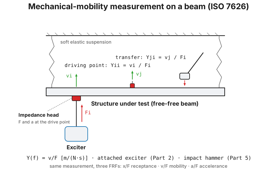
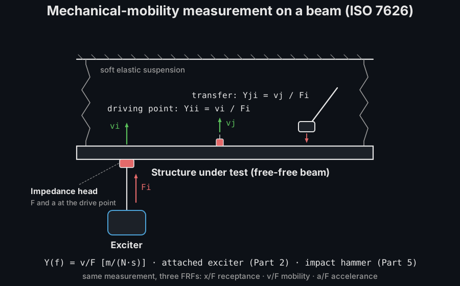
3. Measured FRFs and their acceptance criteria (ISO 7626-2)

In the usual ISO 7626-2 arrangement the structure hangs on a compliant suspension (the standard admits freely suspended or grounded structures; clause 5.2 asks a grounded support to be representative of the intended application), an exciter drives one point through an impedance head (a transducer stack measuring force and acceleration at the same point, which is what gives the attached-exciter setup its driving-point FRF), and accelerometers pick up the response elsewhere for the transfer FRFs. ISO 7626-5 covers the alternative of impact excitation with an exciter that is not attached to the structure, in practice usually an instrumented hammer: it trades the attached exciter’s controlled spectrum for speed, with an excitation spectrum set by the impactor mass and tip stiffness.

What the suspension has to do (clause 5.3)

“Soft enough” is not the criterion; ISO 7626-2 clause 5.3 gives three numbers, and the first of them is a mobility criterion, which is checkable with the functions this page has already introduced.

• The driving-point mobility of the suspension at each attachment point should be at least ten times that of the structure at the same point, over the whole frequency range of interest. This is the requirement that matters, because it is what keeps the suspension out of the answer.
• As a minimum requirement, every rigid-body resonance of the suspended structure shall be below half the lowest frequency of interest — the lowest frequency of interest, not the first elastic mode.
• The masses of suspension components near the structure (hooks, turnbuckles) shall be less than one tenth of the free effective mass of the structure at each frequency of interest.

And four practical rules that go with them: attach near nodal points, found by preliminary testing, so the suspension interacts as little as possible; run the cables normal to the excitation direction where practical, and expect transverse string vibrations to affect the data even then; keep the suspension resonances well away from the structure’s modal frequencies, because shock cords and foam pads carry mass but little damping; and watch the damping the suspension itself adds, which the clause raises as a CAUTION. The suspension used must be described in the test report.

The 10× rule is worth executing rather than quoting. For the resonator of section 2 the worst case is its own peak, where the structure is at its most mobile:

# `vibration` is imported by the figure block above; the blocks of a page
# run in reading order.
f0 = vibration.resonance_frequency(2.0, 8000.0)                   # 10.07 Hz
y_structure = abs(complex(vibration.sdof_mobility(f0, 2.0, 8000.0, 5.0)))
print(round(y_structure, 3))                                      # 0.2 = 1/c

# The suspension seen at the same point, disconnected from the structure:
# a shock cord of 31.6 N/m, whose own mobility is omega / k.
y_suspension = abs(complex(
    vibration.convert_frf(31.6, f0, "dynamic_stiffness", "mobility")))
print(round(y_suspension / y_structure, 1))       # 10.0 -> clause 5.3 met

That cord puts the rigid-body bounce of the 2 kg structure at 0.63 Hz, so the minimum requirement is met with room to spare for any lowest frequency of interest above 1.3 Hz. The mobility rule is the binding one, and it is the same criterion, in the same units, as the exciter-attachment rule below: everything you attach to the structure must be at least ten times more mobile than the structure itself.

Attaching the exciter (clause 6.4.4)

ISO 7626-2 calls exciter attachment “often the most difficult problem encountered when using fixed vibration exciters to measure the mobility of lightweight structures”, and gives it a criterion and a design.

• The restraint criterion. With the exciter and its hardware disconnected from the structure, the lateral and rotational driving-point mobilities of the attachment shall be at least ten times larger, at all frequencies of interest, than the corresponding elements of the structure’s driving-point mobility matrix. An exciter that fails it clamps the structure laterally and rotationally, and the low-order modes are the first casualty.
• The drive rod. High stiffness along the excitation axis and enough flexibility in every other direction: slender short rods are usual, but thick rods with thin flexible sections near each end can do better. Align the exciter and the rod with the force-transducer axis. Two things to watch: drive-rod bending modes inside the frequency range can interfere with the measurement, and bending of the exciter’s own moving system can inject moments the force transducer never sees.
• Where the two transducers go, which is where validity is decided and which the inset of the diagram above draws. With a flexible drive rod the accelerometer shall be attached directly to the structure, never through the rod, whose axial compliance makes the response measurement invalid. The force transducer shall measure the force transmitted from the rod into the structure; putting it at the exciter end is admitted “only with extreme caution”, and then the rod compliance must be checked per ISO 7626-1 and the rod mass compensated by the mass-cancellation procedure below.
• Area-reducing cones may be needed to approximate a point force, and can themselves introduce a spurious moment if used carelessly.

What the transducers do to the answer (clauses 6.4.2, 6.4.3 and 7.3)

Every transducer you attach adds mass, and the spurious force needed to accelerate that mass is measured as though the structure had produced it. The symptom is the damaging part: uncompensated inertia loading shifts the frequencies of the response peaks, and a resonance measured in the wrong place is inherited by everything downstream — the modal fit, the damping from the half-power bandwidth, the $|Y|=1/c$ read of section 2. Rotational inertia does the same to moments (6.4.3), and impedance heads are the worst offenders because their moment of inertia about the mounting point can be large.

The standard’s sequence is: choose the smallest mass and lowest inertia consistent with sensitivity; then, if that is not enough, compensate.

• When to act. Electronic compensation shall be considered when the magnitude of the structure’s driving-point mobility exceeds $0,01/(f{m}_t)$ at all frequencies of interest, with $m_t$ the total effective mass of the attachment hardware plus the effective end mass of the force transducer or impedance head (and of a separate driving-point accelerometer, if one is fitted).
• What it is. “Mass cancellation”: multiply the driving-point acceleration by $m_t$ and subtract the product from the force signal, in analogue or digitally. A transfer-mobility measurement therefore needs a separate accelerometer at the driving point to supply that signal.
• What it cannot do. It compensates translational inertia at the driving point, in the excitation direction, only — never rotational inertia. The standard strongly recommends reconsidering the transducer selection and redesigning the attachment hardware ahead of using it, and confines it to the range where the ratio of attachment-and-transducer effective mass to the structure’s free effective mass at the driving point is between 0,05 and 0,5.
• Clause 7.2 adds the rule that makes any of this repeatable: transducers mounted on studs are tightened to the torque the manufacturer recommends, and attachment compliance is checked per ISO 7626-1.

For the resonator of section 2 the trigger is easy to place. Its driving-point mobility peaks at $1/c=0.2$ m/(N·s) at 10.07 Hz; with a 20 g impedance head and attachment hardware ($m_t=0.02$ kg) the trigger $0,01/(f{m}_t)$ is 0.050 m/(N·s) there, so at its peak the structure is four times above it. Take a 2 g head instead and the trigger rises to 0.50 m/(N·s), above the peak. The trigger falls as the added mass rises, which is the whole point of it: the same structure needs compensation with a heavy transducer and not with a light one.

Processing measured random-excitation records per ISO 7626-2, 8.1.3 (the H1 estimator $\hat{H}=G(\text{response},\text{force})/G(\text{force},\text{force})$) and the ordinary coherence ${\gamma }^2=|G_{xy}{|}^2/(G_{xx}{G}_{yy})$ used for its data-quality checks are the library’s existing spectral estimators transfer_function and coherence (H1 is their default).

Reading the coherence, and the one bias H1 has (Annex A.1)

Annex A.1 is a diagnosis table, and it is the most immediately useful page of the standard. A coherence substantially below 1 says something specific depending on where it drops.

• Notches at the resonances and antiresonances mean inadequate frequency resolution (which also biases the computed FRF), inadequate time-domain weighting, a nonlinear structure or a saturating amplifier, more than one input force, or digitising and electronic noise from an inadequate exciter force.
• Notches at the resonances specifically can also mean the exciter’s force drops there, which is inherent when a shaker drives a lightly damped structure. That leads to the bias worth knowing before recommending H1: if the force signal falls below the noise floor, the H1 estimate — the cross-spectrum over the force auto-spectrum — reads too low, exactly at the resonance peak the reader is being taught to measure the damping from. H2 (response auto-spectrum in the denominator) has the opposite bias, being the one to reach for when the noise is on the force; Hv sits between them. transfer_function provides H1 by default.
• A broad droop across the range is poor signal-to-noise, usually inadequate dynamic range: shape the excitation spectrum, or use synchronous time-domain averaging.
• Low coherence anywhere can simply be nonlinearity.

Two notes catch beginners. A coherence computed from a single record is always a fictitious 1,0, so it means nothing until several averages are in. And a high coherence does not prove the data valid: it can equally indicate cross-talk between the force and response channels.

The acceptance criteria

On top of the estimators, two ISO 7626-2 acceptance criteria are provided:

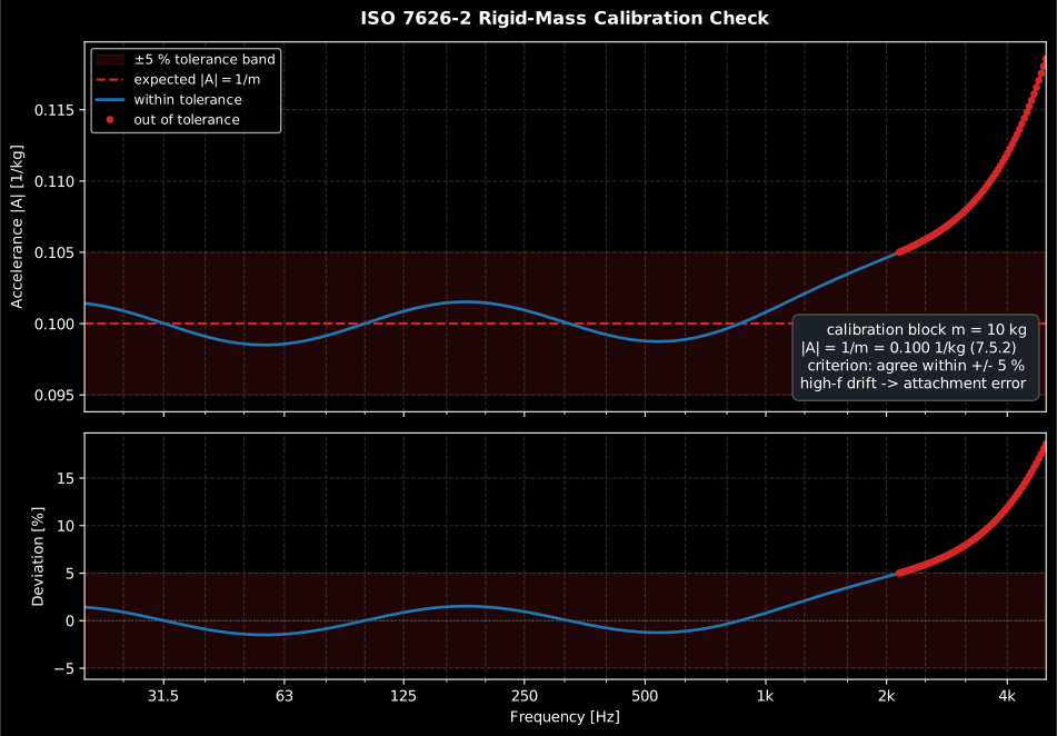
• Operational rigid-mass calibration (7.5.2). The measured FRF of a freely suspended rigid block of known mass must agree within ±5 % with $|A|=1/m$ (accelerance) or $|Y|=1/(2\pi fm)$ (mobility).
• Random error (Annex A + 8.1.3). Enough spectra must be averaged that the normalized random error $\epsilon =\sqrt{(1-{\gamma }^2)/(2n{\gamma }^2)}$ at each resonance of a driving-point mobility is below 5 %.

import numpy as np
from phonometry import vibration

# A 10 kg calibration block: |A| must be 1/m = 0.100 1/kg at every frequency.
f = np.array([20.0, 100.0, 500.0])
res = vibration.rigid_mass_calibration_check([0.100, 0.102, 0.097], f, mass=10.0)
print(res.passed, res.within_tolerance.tolist())   # True [True, True, True]

# The Annex A example: coherence 0.8 needs about 75 averages for < 5 %.
print(round(float(vibration.random_error_percent(0.8, 75)), 2))   # 4.08  %

The random-error criterion is a decision taken before a measurement, not a check after one, and how many averages it costs depends steeply on the coherence you expect:

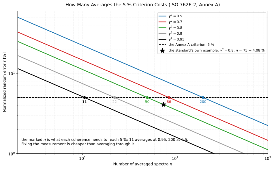
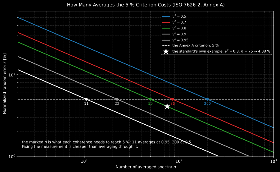
What the criterion costs, as a function of how good the measurement already is. Reaching 5 % takes 11 averages at ${\gamma }^2=0.95$ and 200 at ${\gamma }^2=0.5$ — a factor of twenty for a factor of two in coherence. That is the argument for fixing the measurement, with the Annex A.1 diagnosis above, rather than averaging through it.

Show the code for this figure

import matplotlib.pyplot as plt
import numpy as np

averages = np.unique(np.round(np.logspace(np.log10(2.0), np.log10(1000.0), 260)))
for coherence in (0.5, 0.7, 0.8, 0.9, 0.95):
    error = [float(vibration.random_error_percent(coherence, int(n)))
             for n in averages]
    plt.loglog(averages, error, label=f"coherence {coherence}")
    # The n at which this coherence reaches the 5 % criterion.
    print(coherence, round((1.0 - coherence) / (2.0 * coherence * 0.05**2)))
plt.axhline(5.0, ls="--", color="0.4")
plt.xlabel("Number of averaged spectra"); plt.ylabel("Random error [%]")
plt.legend(); plt.show()

Three more tests the standard asks for, and this page does not run

Clause 10 is explicit that the Annex A.1 averaging procedure applies to random excitation, and that “additional tests, applicable to all types of excitation, are described in A.2 to A.4”. Those three are not implemented here, but they are cheap, and a measurement that has passed only the two criteria above is not yet validated.

• A.2, linearity. Bolted joints, support clearances and similar features make practical structures nonlinear. Measure the FRF, then repeat it with the excitation amplitude significantly increased and significantly decreased; if the results disagree, the reason needs further analysis. The clause asks for this in the course of each test series, and it is the check that catches what a coherence notch only hints at.
• A.3, reciprocity. For a linear elastic structure $Y_{ij}(f)=Y_{ji}(f)$: swap the exciter and the response accelerometer and the transfer mobility must come back the same. It is a strong end-to-end test of the whole chain, including the attachment restraints above, and it costs one extra measurement. (Some elements, hydrodynamic bearings among them, are genuinely non-reciprocal; between such an element and the drive point the test does not apply.)
• A.4, driving point against transfer. The phase and antiresonance checks of section 2: a driving-point FRF stays inside $\pm 90°$ and shows an antiresonance between every pair of resonances.

The distinction is worth keeping: A.1 is a precision criterion, answering how many averages a given random error costs, while A.2 to A.4 are validity criteria that no amount of averaging will fix.

The calibration check returns a RigidMassCalibrationResult carrying the per-frequency deviation and pass flags, and a .plot(): the measured FRF magnitude against the rigid-mass line with its ±5 % tolerance band (upper panel) and the relative deviation against the same band (lower panel, where a few-percent tolerance is actually readable). A calibration that drifts out of the band towards a few kHz points at a transducer or attachment-compliance error, exactly what the check is meant to catch:

import numpy as np
from phonometry import vibration

m = 10.0                                                  # calibration block mass
f = np.logspace(np.log10(20.0), np.log10(5000.0), 400)
drift = 0.05 * (f / 2500.0) ** 2                          # high-frequency drift
measured = (1.0 / m) * (1.0 + 0.015 * np.sin(2 * np.pi * np.log10(f)) + drift)
res = vibration.rigid_mass_calibration_check(measured, f, mass=m)
print(res.passed)                                         # False (drift exceeds 5 %)
res.plot()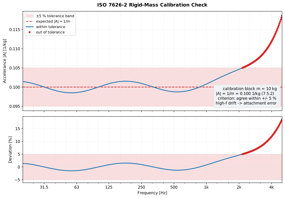

Show the code for this figure

import matplotlib.pyplot as plt
import numpy as np
from phonometry import vibration

m = 10.0
f = np.logspace(np.log10(20.0), np.log10(5000.0), 400)
drift = 0.05 * (f / 2500.0) ** 2
measured = (1.0 / m) * (1.0 + 0.015 * np.sin(2 * np.pi * np.log10(f)) + drift)
res = vibration.rigid_mass_calibration_check(measured, f, mass=m)
bad = ~res.within_tolerance

fig, (top, bot) = plt.subplots(2, 1, sharex=True, figsize=(10, 7),
                               gridspec_kw={"height_ratios": [1.5, 1.0]})
top.fill_between(f, res.expected * 0.95, res.expected * 1.05, color="C1",
                 alpha=0.15, label="±5 % tolerance band")
top.semilogx(f, res.expected, "--", color="C1", label="expected |A| = 1/m")
top.semilogx(f, res.measured, color="C0", label="within tolerance")
top.semilogx(f[bad], res.measured[bad], "o", color="C1", label="out of tolerance")
top.set_ylabel("Accelerance |A| [1/kg]"); top.legend()

bot.axhspan(-5.0, 5.0, color="C1", alpha=0.15)
bot.semilogx(f, 100.0 * res.deviation, color="C0")
bot.semilogx(f[bad], 100.0 * res.deviation[bad], "o", color="C1")
bot.set_xlabel("Frequency [Hz]"); bot.set_ylabel("Deviation [%]")
plt.show()

4. The MobilityResult bundle

sdof_mobility_result bundles the FRF over frequency into a MobilityResult, which exposes .magnitude, .phase, .to(target) (any Table-1 kind) and a .plot() of $|Y(f)|$ with the resonance marked:

import numpy as np
from phonometry import vibration

f = np.logspace(np.log10(0.5), np.log10(200.0), 400)
res = vibration.sdof_mobility_result(f, mass=2.0, stiffness=8000.0, damping=5.0)
z = res.to("impedance")                        # impedance = 1/Y per frequency
print(res.frequencies[int(np.argmax(res.magnitude))].round(1))   # ~10.1 Hz

res.plot()   # |Y(f)| with the resonance marked (needs matplotlib)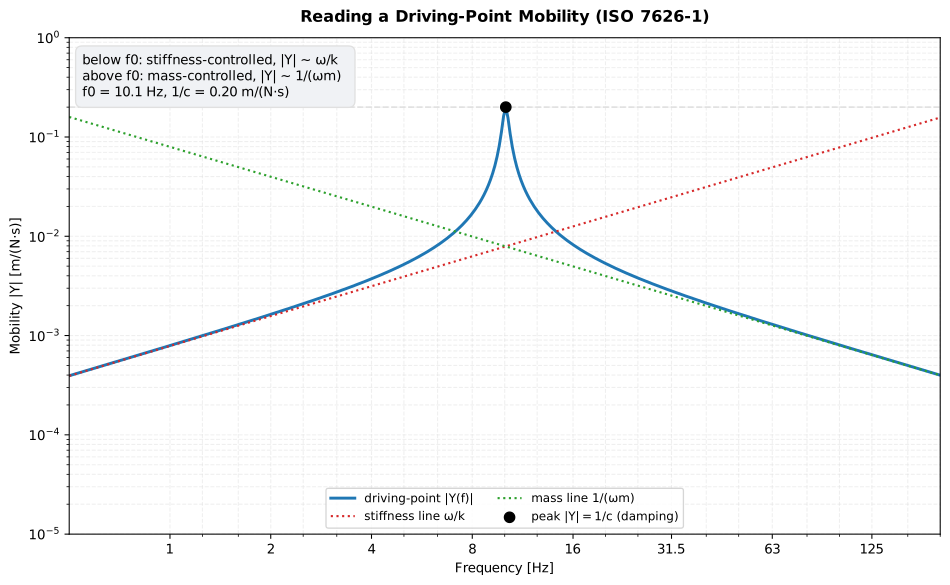

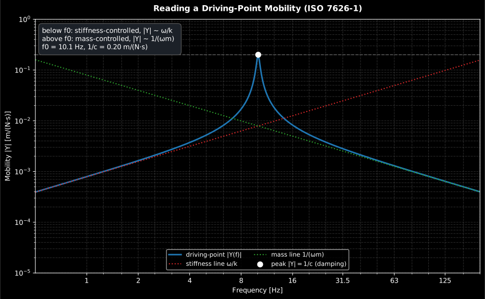
Reading a driving-point mobility is a structural diagnosis. Below the resonance the magnitude climbs along the stiffness line $\omega /k$, above it it falls along the mass line $1/(\omega m)$, and the height of the peak between them is $1/c$ — a direct read of the damping, for this isolated resonator; on a real structure with overlapping modes the damping is estimated by modal fitting or from the half-power bandwidth instead. The lower panel is the same statement in phase: $+90°$ on the stiffness line, $-90°$ on the mass line, and exactly $0°$ at the resonance, which is what “purely real” means and why the peak equals $1/c$.

Show the code for this figure

import matplotlib.pyplot as plt
import numpy as np
from phonometry import vibration

m, k, c = 2.0, 8000.0, 5.0
f = np.logspace(np.log10(0.5), np.log10(200.0), 400)
res = vibration.sdof_mobility_result(f, mass=m, stiffness=k, damping=c)

# One line — |Y(f)| with the resonance marked:
res.plot()
plt.show()

# By hand, adding the stiffness and mass asymptotes the prose describes:
w = 2.0 * np.pi * f
fig, ax = plt.subplots()
ax.loglog(f, res.magnitude, label="driving-point |Y(f)|")
ax.loglog(f, w / k, ":", label="stiffness line ω/k")
ax.loglog(f, 1.0 / (w * m), ":", label="mass line 1/(ωm)")
ax.axhline(1.0 / c, ls="--", color="0.6", label="peak |Y| = 1/c")
ax.set_xlabel("Frequency [Hz]")
ax.set_ylabel("Mobility |Y| [m/(N·s)]")
ax.set_title("Reading a driving-point mobility (ISO 7626-1)")
ax.legend()
plt.show()

5. Reference mobilities when nothing has been measured

The SDOF is a reference for the definitions, not a model of anything a building acoustician owns. For a large plate or a long beam, driven away from its edges, the reflected waves that make a real structure resonate have decayed before they return, and the driving-point mobility takes the closed form of the equivalent infinite structure — which is exactly the stand-in EN 12354-5 wants for a receiver mobility when no measurement exists. Three characters, from Cremer, Heckl & Petersson Table 5.1:

• the infinite plate is a pure real resistance, $Y=1/(8\sqrt{B^{\prime }{m}^{\prime \prime }})$, independent of frequency: it absorbs at every frequency alike and has no peak to read a damping from;
• the infinite beam is $Y=(1-\mathrm{j})/(4m^{\prime }{c}_B)$, so $-45°$ of phase at every frequency and a magnitude falling as ${\omega }^{-1/2}$, because the bending wave speed $c_B$ itself grows as $\sqrt{\omega }$;
• a rod in longitudinal motion is $Y=1/(\rho c_{L}S)$, real and flat again — the mechanical analogue of a matched transmission line.

import numpy as np

f = np.array([50.0, 500.0])

# A 140 mm concrete slab: E = 30 GPa, nu = 0.2, rho = 2400 kg/m3.
b_plate = vibration.plate_bending_stiffness(3.0e10, 0.14, 0.2)
plate = vibration.infinite_plate_point_mobility(f, b_plate, 336.0)
print(f"{float(plate.magnitude[0]):.3e}", round(float(np.degrees(plate.phase[0]))))
#  2.551e-06 0     -> real, and the same at 500 Hz

# A 100 x 200 mm steel beam, driven at a point away from its ends.
b_beam = 2.1e11 * 0.1 * 0.2**3 / 12.0
beam = vibration.infinite_beam_point_mobility(f, b_beam, 7800.0 * 0.02)
print(f"{float(beam.magnitude[0]):.3e}", round(float(np.degrees(beam.phase[0]))))
#  7.388e-06 -45
print(np.round(vibration.beam_bending_wave_speed(f, b_beam, 7800.0 * 0.02), 1))
#  [306.8 970.1]  -> c_B grows as sqrt(f), so |Y| falls as 1/sqrt(f)

Both constructors return a MobilityResult, so they plot, convert with .to() and report exactly like the SDOF above. Two more cover the degrees of freedom the pair does not: infinite_beam_moment_mobility is the rotational mobility a junction line or a bracket bolted at two points needs, in rad/(N·m·s), for when the excitation is a moment rather than a force; and longitudinal_rod_mobility (with its longitudinal_rod_impedance reciprocal) covers a strut or a pipe run loaded along its axis.

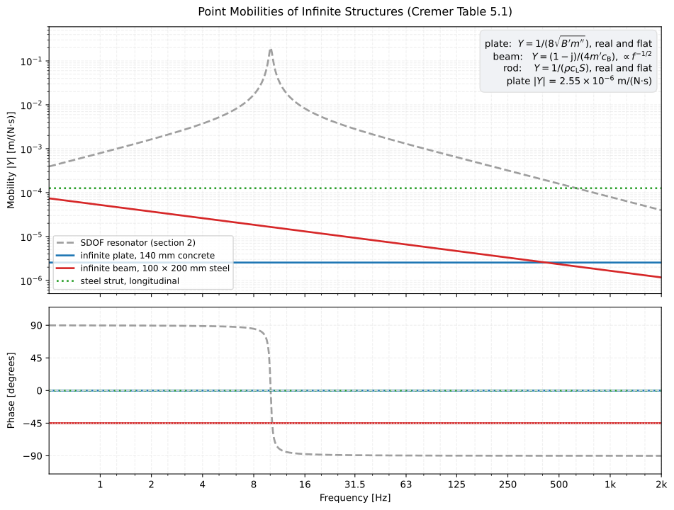
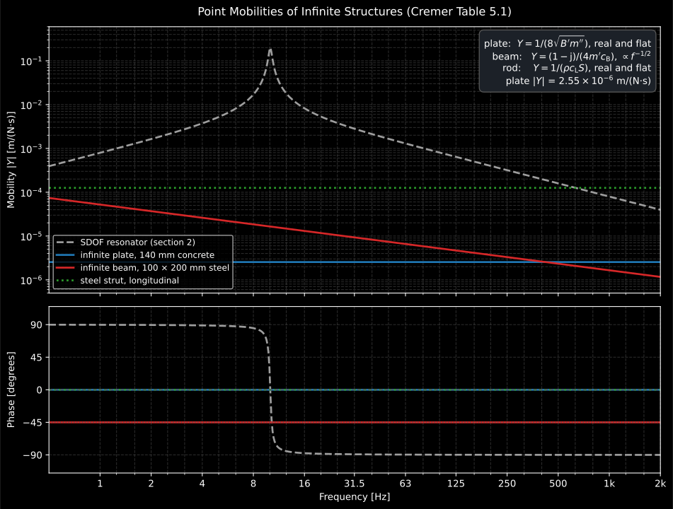
The contrast the whole section is for. An infinite structure never reflects anything back, so it has no resonance and no peak: the plate and the rod are real and flat, the beam falls as $f^{-1/2}$ at a constant $-45°$. Reading a mobility plot as “stiffness line, peak, mass line” is a statement about finite structures; a large plate is the case where none of the three appears.

# One line each, on shared axes with the SDOF of section 4.
plate.plot()
beam.plot()

Where do these numbers go? Into panel sound insulation, which uses the same functions to price a panel’s radiation, and into the EN 12354-5 receiver mobility of installed structure-borne sound.

Test-report fiche

MobilityResult.report(path) renders a one-page mechanical-mobility measurement report (ISO 7626-1:2011 FRF definitions, measurement per ISO 7626-2:2015). Mobility is a continuous frequency-response function, not an octave-band quantity, so the sheet presents it honestly as the $|Y(f)|$ magnitude spectrum plus a compact table of characteristic points (the FRF type, driving-point or transfer, the frequency range, the peak frequency, the peak mobility magnitude and the phase there), and a boxed peak mobility $|Y|$ at the frequency it occurs at (for a driving-point FRF a resonance, where $|Y|=1/c$ measures the damping). It is a characterisation, so there is no pass/fail verdict; language="es" renders the Spanish fiche. The fiche always embeds the $|Y(f)|$ spectrum, so it needs both the report and plot extras (pip install "phonometry[report,plot]").

from phonometry import ReportMetadata, vibration

res = vibration.sdof_mobility_result(f, mass=2.0, stiffness=8000.0, damping=5.0)
res.report(
    "mobility.pdf",
    metadata=ReportMetadata(
        specimen="Machine support bracket (driving point)",
        measurement_standard="ISO 7626-2",
    ),
)   # one-page fiche (needs phonometry[report,plot])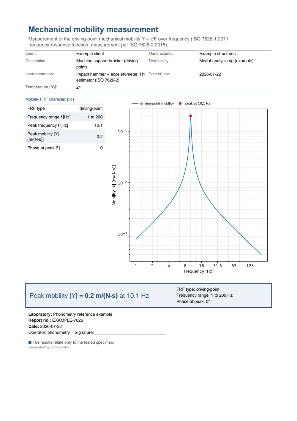

One-page mechanical-mobility fiche: a metadata header, a table of the FRF characteristic points (the FRF type, the frequency range, the peak frequency, the peak mobility magnitude and the phase there) beside the mobility magnitude spectrum, and the boxed peak mobility.

Download the report (PDF)

Mechanical-mobility fiche (MobilityResult.report): the FRF characteristic points and the mobility magnitude spectrum.

What this guide covers

• Covered

  ISO 7626-1:2011’s FRF family (Table 1): receptance, mobility and accelerance, with their force-per-motion reciprocals, moved between through convert_frf. Also covered are the driving-point/transfer distinction and the closed-form SDOF resonator used as their reference (sdof_receptance, sdof_mobility, sdof_accelerance, resonance_frequency, sdof_mobility_result), and the infinite-structure point mobilities that stand in for a real plate, beam or strut (infinite_plate_point_mobility, infinite_beam_point_mobility, infinite_beam_moment_mobility, longitudinal_rod_mobility and their impedance reciprocals, with plate_bending_stiffness and beam_bending_wave_speed). On the measurement side, ISO 7626-2:2015’s H1 processing of random excitation is covered too (transfer_function, coherence, shared with the electroacoustics guide), along with two acceptance criteria: the 7.5.2 rigid-mass operational calibration (rigid_mass_calibration_check) and the Annex A random-error criterion (random_error_percent).

• Not covered

  ISO 7626-5 covers impact-hammer excitation as an alternative to the attached exciter. It is named here for context only: no function synthesizes or processes an impact-excitation spectrum. The blocked matrix quantities of Table 1, needed for multi-coordinate systems, are not built either. convert_frf returns only the element-wise free reciprocals of ISO 7626-1, 3.1.4, correct for driving-point or single-path use but not for a full FRF matrix. Of the acceptance procedure, only the two criteria above are computed: the clause 5.3 suspension rules, the clause 6.4.4 exciter-attachment criterion, the clause 7.3 mass-cancellation trigger and the A.2 to A.4 linearity, reciprocity and driving-point tests are described here and left to the operator, in the same way ISO 10846’s Inequality 3 is described but not computed on the transfer-stiffness page.

See also

• Transfer stiffness of resilient elements (ISO 10846): the blocked-force limit of section 1, applied to characterise an isolator.
• Structure-borne sound power of equipment (EN 15657): where a source’s mobility and free velocity become an installed power.
• Installed structure-borne sound (EN 12354-5): the prediction that consumes a receiver mobility, measured or taken from section 5.
• Bending-wave transmission at plate junctions: what the plate mobilities of section 5 become at a junction between two of them.
• Frequency response and coherence: the transfer_function and coherence estimators section 3 runs on.
• API reference: vibration.structural.mechanical_mobility.
• Theory: Point mobilities and radiation efficiency: the infinite-structure point mobilities and the radiation efficiency, and why they are averages a finite structure oscillates about.

References

• Cremer, L., Heckl, M., & Petersson, B. A. T. (2005). Structure-borne sound: Structural vibrations and sound radiation at audio frequencies (3rd ed.). Springer. https://doi.org/10.1007/b137728The standard monograph on structural vibration: point and transfer mobilities of beams and plates, and the power flow P = ½·Re{Y}·|F|² that makes mobility the working quantity of this page. ISBN 978-3-540-22696-3.
• International Organization for Standardization. (2011). Mechanical vibration and shock — Experimental determination of mechanical mobility — Part 1: Basic terms and definitions, and transducer specifications (ISO 7626-1:2011). The FRF family and its reciprocals (Table 1, the 3.1.2 mobility and 3.1.4 free-quantity definitions), the free/blocked distinctions and the driving-point / transfer distinction implemented here. Conformance is anchored on the closed-form SDOF identities consistent with those definitions: the driving-point mobility peak |Y(ω0)| = 1/c, the static receptance H(0) = 1/k and the exact Table-1 reciprocity impedance·mobility = 1.
• International Organization for Standardization. (2015). Mechanical vibration and shock — Experimental determination of mechanical mobility — Part 2: Measurements using single-point translation excitation with an attached vibration exciter (ISO 7626-2:2015). The measurement side: the 8.1.3 H1 processing of random excitation, the 7.5.2 rigid-mass operational calibration (±5 %) and the Annex A random-error criterion (< 5 % at resonances). Conformance is anchored on the rigid-mass calibration values (|A| = 0.100 1/kg for 10 kg; |Y| = 1.59155e-4 m/(N·s) at 100 Hz) and the Annex A example (γ² = 0.8, n = 75 → ε = 4.08 %).