Predicting vibration before measuring (DIN 4150-1)
Standards: DIN 4150
Part 1 of DIN 4150 is the first question of the series. Before a quarry is blasted, a chimney felled, a pile driven or a line built, someone has to say how much vibration will reach the houses and how much of it the floors will feel, and Part 1 gives the shapes of every answer. It gives no recipe, and says so in its foreword: the constants of a real case come from trial blasts, from comparable ground, from a measurement with a few machines running. What it does fix, it fixes plainly, and its Annex A shows the shapes in the ground twenty-seven times over.
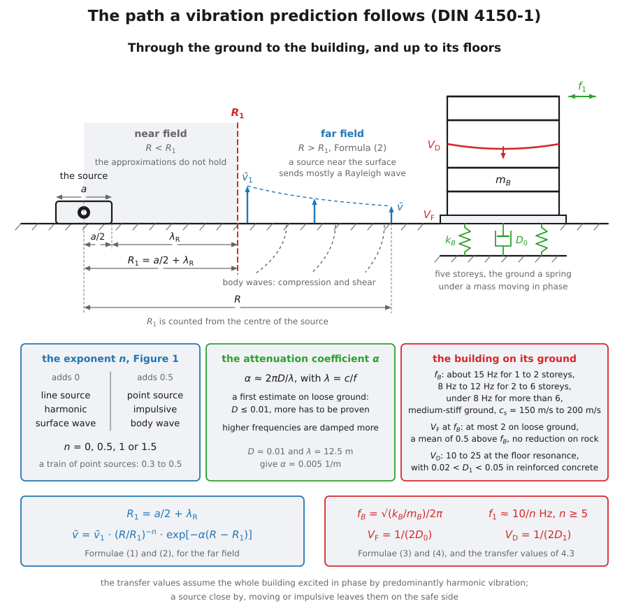
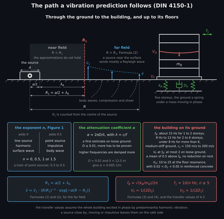
The path clause 4 of Part 1 lays down for propagation and transfer: a near field where its approximations do not hold, the decay of Formula (2) beyond it, and a building that sits on its ground as a mass on a spring and hands the motion on through its foundation to its floors.
1. How far vibration carries
Section titled “1. How far vibration carries”Every source has a near field and a far field, and the boundary is
R₁ = a/2 + λ_R (Formula (1)): half the extent of the source along the
direction of propagation plus a wavelength of the surface wave. Nearer than
that nothing here holds. Beyond it the velocity amplitude decays as
v = v₁ · (R / R₁)^-n · exp[-α (R - R₁)](Formula (2)): geometric spreading with an exponent n that Figure 1 fixes
by three yes-or-no questions, and material damping with
α ≈ 2π D / λ, the damping ratio of the ground over the wavelength that
matters. The exponent is 0 for a harmonic line source carried by a surface
wave and gains 0,5 for each of point instead of line, impulsive instead of
harmonic, and body wave instead of surface wave, up to 1,5 for an impulsive
point source in a body wave. A train is a chain of point sources not
excited in phase and decays with something between 0,3 and 0,5. For loose
ground a first estimate may take a damping ratio of 0,01 at most; more has
to be proven.
from phonometry import vibration
print(vibration.geometric_exponent(geometry="point", character="impulsive", wave="surface"))  # 1.0print(vibration.geometric_exponent(geometry="line", character="harmonic", wave="surface"))  # 0.0print(vibration.reference_distance_m(6.0, rayleigh_wavelength_m=12.5))  # 15.5
# Annex A, Figure A.19: a machine hall measured at 0,44 mm/s 13 m away,# with D = 0,01 and a wavelength of 12,5 m.alpha = vibration.attenuation_coefficient_per_m(0.01, wavelength_m=12.5)print(f"{alpha:.4f} 1/m")  # 0.0050 1/mdecay = vibration.far_field_velocity_mm_s(    0.44, [20.0, 40.0, 80.0], reference_distance_m=13.0, exponent=1.0, attenuation_per_m=alpha)print(decay.round(3))  # [0.276 0.125 0.051]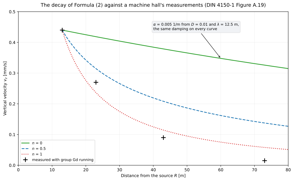
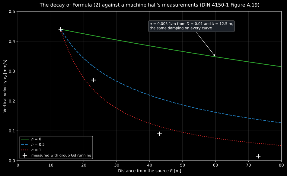
Figure code
import matplotlib.pyplot as pltimport numpy as np
from phonometry import vibration
distances = np.linspace(13.0, 80.0, 200)fig, ax = plt.subplots(figsize=(10, 6.2))for exponent in (0.0, 0.5, 1.0):    ax.plot(        distances,        vibration.far_field_velocity_mm_s(            0.44, distances, reference_distance_m=13.0, exponent=exponent, attenuation_per_m=0.005        ),        label=f"$n$ = {exponent:g}",    )ax.plot([13.0, 23.0, 43.0, 73.0], [0.44, 0.27, 0.09, 0.015], "k+", markersize=11, label="measured")ax.set_xlabel("Distance [m]")ax.set_ylabel("Vertical velocity [mm/s]")ax.legend()
The damping alone is worth drawing, and Figure 2 draws it for a damping ratio of 0,01 and a wave speed of 200 m/s: over 100 m the ground takes 27 % of the amplitude at 10 Hz and 79 % at 50 Hz, which is why the low frequencies are what arrives at a distance.
from phonometry import vibration
for frequency in (10.0, 50.0):    left = vibration.material_damping_factor(        [100.0], damping_ratio=0.01, frequency_hz=frequency, wave_speed_m_s=200.0    )[0]    print(f"{frequency:g} Hz: {left:.3f} of the amplitude left after 100 m")# 10 Hz: 0.730 of the amplitude left after 100 m# 50 Hz: 0.208 of the amplitude left after 100 m
2. Into the building, and up the floors
Section titled “2. Into the building, and up the floors”A building on the ground is a mass on a spring, with the natural frequency
of Formula (3), f_B = √(k_B / m_B) / 2π, for the vertical direction and
predominantly harmonic vibration: about 15 Hz for one or two storeys, 8 Hz
to 12 Hz for two to six, under 8 Hz above that, on a ground of medium
stiffness with a shear wave speed of 150 m/s to 200 m/s. At that frequency
the foundation passes at most 1 / (2 D₀) of the ground’s amplitude, and
for loose ground D₀ may be taken as 0,25, so the foundation amplifies by
2 at most; above it a mean transfer of 0,5 may be assumed, and on rock there
is no reduction at all. A floor then amplifies by at most 1 / (2 D₁) at its
own resonance, 10 to 25 for a concrete floor with a damping ratio between
0,05 and 0,02, on the assumption that the building is excited in phase over
its whole footprint, which is the safe side for a source that is close,
moving or impulsive. And the lowest horizontal natural frequency of a
building of five storeys or more is about 10 / n Hz (Formula (4)), which
matters where a tall slender building meets a low excitation frequency.
from phonometry import vibration
print(f"{vibration.soil_building_natural_frequency_hz(2.5e9, mass_kg=4.0e5):.1f} Hz")  # 12.6 Hzprint(vibration.soil_building_frequency_guide_hz(4))  # (8.0, 12.0)print(vibration.foundation_transfer_max())  # 2.0print(f"{vibration.floor_transfer_max(0.03):.1f}")  # 16.7print(vibration.storey_frequency_hz(8))  # 1.25
3. Single events: a blast and a falling mass
Section titled “3. Single events: a blast and a falling mass”In the far field a blast follows v_max = k (L/L₀)^b (R/R₀)^-m (Formula (5))
with the charge per delay L against 1 kg, the distance against 1 m, and
three constants that come from trial blasts or from comparable cases in
ground, method and range of distance, with allowance for scatter; the
standard prints none of them. A falling mass follows the same with the
root of its fall energy G · h (Formula (6)), which for a felled chimney is
usually the larger source, the demolition blast the smaller. Quarry
blasting is very rarely relevant beyond 1500 m, construction blasting
beyond 400 m.
from phonometry import vibration
# Constants of the user's own trial blasts; the standard prints none.peak = vibration.blast_peak_velocity_mm_s(    50.0, [300.0, 600.0], coefficient_mm_s=1200.0, charge_exponent=0.6, distance_exponent=1.7)print(peak.round(2))  # [0.77 0.24]
# A 2 600 t chimney, its centre of mass 70 m up: 25 506 kN through 70 m.energy = vibration.fall_energy_kj(25506.0, drop_height_m=70.0)print(f"{energy:.0f} kJ")  # 1785420 kJimpact = vibration.impact_peak_velocity_mm_s(energy, [50.0, 150.0], coefficient_mm_s=0.02, distance_exponent=1.0)print(impact.round(1))  # [0.5 0.2]
4. What a track and a hall of machines excite at
Section titled “4. What a track and a hall of machines excite at”A train excites the ground at its speed over the spacing of whatever repeats along the track or around the wheel, the sleepers first at 0,6 m to 0,9 m, and at the multiples of that, while the parts of the vehicle keep their own frequencies whatever the speed: the car body on its secondary suspension at 1 Hz to 3 Hz, the bogie on its primary at 6 Hz to 10 Hz. Ballasted track passes 40 Hz to 80 Hz on preferentially, a tunnel with under-ballast mats 15 Hz to 40 Hz, a mass-spring system 5 Hz to 20 Hz, and rail vibration reaches about 80 m, further on soft layers.
from phonometry import vibration
print(vibration.track_excitation_frequency_hz(80 / 3.6, spacing_m=0.6, harmonics=2).round(1))  # [37.  74.1]print(vibration.TRACK_TRANSMITTED_BANDS_HZ["ballast"])  # (40.0, 80.0)
A hall of similar machines running together gives, at a point outside,
v_N = χ · v_B · √N (Formula (7)): the velocity measured with N_B of them
running, scaled to N with a correction χ that the standard prints only
as a nomogram, Figure 3, for measurements made with 3, 5, 10, 30, 60 or 100
machines. The nomogram is here as its six curves read off the page at a
five-hundredth, the width of their stroke, and the standard’s own check of
it, Figure A.18, drawn for a hall measured at 0,44 mm/s with three machines
running, is reproduced within 6 %: the measurements follow the curve up to
about sixty machines, the nearest group, and stay flat beyond, because the
groups added after that are further off.
from phonometry import vibration
print(vibration.machine_count_correction([12.0], reference_count=3).round(3))  # [0.448]print(vibration.machine_hall_velocity_mm_s(0.44, [12.0, 44.0, 56.0], reference_count=3).round(2))# [0.68 0.89 0.97], against 0.57, 0.95 and 1.04 measured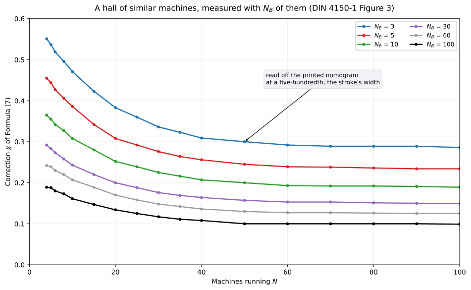
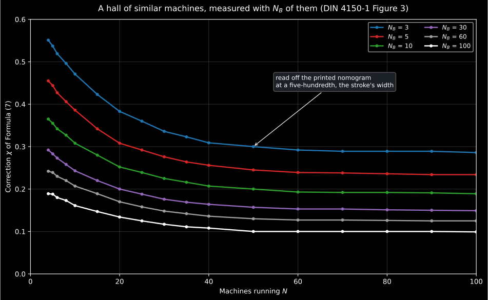
Figure code
import matplotlib.pyplot as plt
from phonometry import vibration
fig, ax = plt.subplots(figsize=(10, 6.2))for reference, chi in vibration.MACHINE_COUNT_CORRECTION.items():    ax.plot(vibration.MACHINE_COUNT_AXIS, chi, marker="o", markersize=3, label=f"$N_B$ = {reference}")ax.set_xlabel("Machines running")ax.set_ylabel(r"Correction $\chi$")ax.legend(ncol=2)
5. Four things printed wrong
Section titled “5. Four things printed wrong”The symbol lists of Formulae (5) and (6) give the distance in millimetres
against a reference of one metre, which Formula (2) and every axis of Annex
A say is metres. Clause 5.2.3 speaks of vibratory drivers with a low working
frequency and writes f > 30 Hz, the sign the wrong way round after a
paragraph that calls the high frequencies above 35 Hz the favourable ones.
Figure A.2’s legend gives the continuous line to the vertical component and
the dash-dot line to the radial one, and the drawing has them the other way
about. A.5.1 prints an eccentric moment in newtons. And the sixth measured
point of Figure A.18, labelled all groups of a hall of 252 machines, sits at
110, the count of the groups of the hall nearest the measuring point. The
errata page has all five with their pages.
Propagation: the far-field boundary of Formula (1), the decay of Formula (2) with the exponents of Figure 1 and the damping of the ground, and the damping factor of Figure 2 on its own.
The building: the natural frequency of Formula (3) and its guide values by storeys, the transfer of a foundation and a floor at resonance, and the storey formula of Formula (4). The sources: the blast and the falling mass of Formulae (5) and (6), the machine hall of Formula (7) with the nomogram of Figure 3 read off the page, the excitation frequencies of a track, and the frequency bands, ranges and constants Clause 5 gives its sources.
Not covered
No constants for a real case. The
k,bandmof a blast and thekandmof an impact are the user’s; the standard prints none and the library carries none. The measured cases of Annex A are described in the standard and not reproduced here, and its two figures drawn from the formulas are held as conformance rows, not offered as data.No near field. Nearer than
R₁the standard asks for a numerical or experimental investigation of its own, and the library refuses the distance.
What this guide covers
Section titled “What this guide covers”References
Section titled “References”- Deutsches Institut für Normung. (2001). Erschütterungen im Bauwesen — Teil 1: Vorermittlung von Schwingungsgrößen (DIN 4150-1:2001-06). Formulae (1) to (7), the exponents of Figure 1, the damping curves of Figure 2, the nomogram of Figure 3 read off the page, and the guide values and frequency bands Clauses 4 and 5 give for the ground, the building and each kind of source. The measured cases of Annex A are described, not implemented; Figures A.18 and A.19, which the standard draws from Formulae (7) and (2) with every parameter printed, are the conformance rows.